All published articles of this journal are available on ScienceDirect.

Online Seizure Prediction System: A Novel Probabilistic Approach for Efficient Prediction of Epileptic Seizure with iEEG Signal
Abstract
Background:
1% of people around the world are suffering from epilepsy. It is, therefore crucial to propose an efficient automated seizure prediction tool implemented in a portable device that uses the electroencephalogram (EEG) signal to enhance epileptic patients’ life quality.
Methods:
In this study, we focused on time-domain features to achieve discriminative information at a low CPU cost extracted from the intracranial electroencephalogram (iEEG) signals of six patients. The probabilistic framework based on XGBoost classifier requires the mean and maximum probability of the non-seizure and the seizure occurrence period segments. Once all these parameters are set for each patient, the medical decision maker can send alarm based on well-defined thresholds.
Results:
While finding a unique model for all patients is really challenging, and our modelling results demonstrated that the proposed algorithm can be an efficient tool for reliable and clinically relevant seizure forecasting. Using iEEG signals, the proposed algorithm can forecast seizures, informing a patient about 75 minutes before a seizure would occur, a period large enough for patients to take practical actions to minimize the potential impacts of the seizure.
Conclusion:
We posit that the ability to distinguish interictal intracranial EEG from pre-ictal signals at some low computational cost may be the first step towards an implanted portable semi-automatic seizure suppression system in the near future. It is believed that our seizure prediction technique can conceivably be coupled with treatment techniques aimed at interrupting the process even prior to a seizure initiates to develop.
1. INTRODUCTION
According to the UN’s World Health Organization (WHO), epilepsy affects more than 70 million people worldwide [1 -3] and epilepsy, as the fourth most prevalent neurological disorder, follows migraine, stroke, and Alzheimer [2]. The epileptic patients suffer from unexpected recurrent seizures, which are indirectly linked to their quality of lives, including loss of consciousness, mental illness, strange sensations, depression, and convulsions. If seizures are not controlled, these patients have to deal with major limitations in family, social, educational, and vocational activities [4]. Epilepsy can be treated with medication or surgery procedures, but poor response to medication remains a serious limitation in the treatment of epileptic seizures. If the seizures are not managed successfully, they can restrict the patient’s lifestyle. In these scenarios, individuals may not independently work and have some activities [4-6] since they are vulnerable to face severe issues like injuries and sudden death, limited independence, restrictions in driving, and having troubles finding and keeping a job. Then forecasting the seizure enough in advance will considerably enhance the patient’s life quality [7, 8].
The increased use of Implantable Medical Devices (IMDs) in all aspects of medicine makes them a suitable candidate in both clinical trials and for ongoing epilepsy management [2, 9, 10]. Anti-seizure devices, like Deep Brain Stimulator (DBS) [11] and Vagus Nerve Stimulator (VNS) [12], have been explored and implemented to decrease significantly the seizure frequency for individuals who have not treated with Anti-Epileptic Drugs (AED) [5, 13, 14]. These implanted devices interrupt and stimulate nerve activity by carrying electrical impulses to a specific target area. On the other hand, these devices carry chronic therapy instead of a smart targeted therapy as well as suffer from the physiological feedback which delimits their efficacy [14]. Over the past 80 years, studying ElectroEncephaloGraphy (EEG), either invasive or non-invasive, is an entrenched methodology in evaluating the electrical activity of the brain and in unraveling the physiological process of the seizure [7, 15].
With the advance of machine learning algorithms, scholars are striving towards hiring these approaches to advance clinical practice. The machine learning models require a number of features to serve the algorithm as inputs [16]. Features are variables that can represent the changes of a signal and for the last decades, scholars have demonstrated that various types of features have the predictability of impending seizures, which can vary from interictal (no seizure) to pre-ictal phase (period before a seizure) [2, 17]. Therefore, a machine-learning algorithm with a closed-loop electrical stimulation and automated anti-epileptic medicines will be a suitable solution to tackle the above problems. On demand medicine and therapy medical equipment that can take an action prior to a seizure will also help to minimize the devastating side effects induced by regular usage of AEDs [18].
In spite of extensive studies in the field of seizure prediction, the severity and future occurrence of epileptic seizure attacks are hard to be anticipated [9] and even the complexity, non-linearity, and uncertainty of the EEG data make it challenging to develop a highly generic seizure prediction framework across all patients [7].
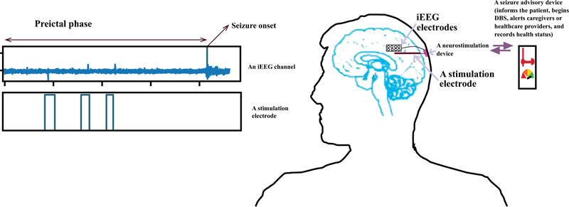
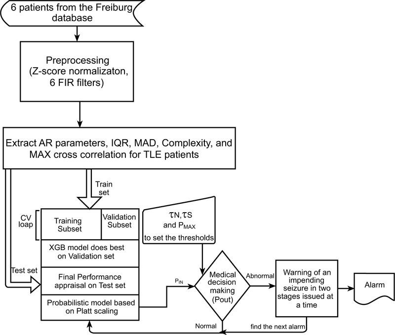
A more systematic and logical approach to deal effectively with this issue is to collect long-term continuous EEG data and make an adaptive machine learning model (an automated labeling and training) with an adaptive seizure warning system [19] which can be the subject of ongoing research in the future. Fig. (1) demonstrates a semi-autonomous closed loop seizure prevention system. AED or DBS are generally employed to suppress from happening and reduce the severity of the seizures, although they do not affect the normal functionality of the brain. Nevertheless, they do not cure seizures and are just a tool for long-term management of epilepsy [20-22].
To this end, in this research, we posit a new probabilistic seizure prediction approach with some time-domain features recommended to achieve discriminative information at a low computational cost [23].
One of the limitations of published articles in this area is about using limited data in their research. The researchers endeavored to investigate just one minute of data [24, 25], they employed a limited amount of data: 5 min preictal and 10 min interictal. Additional remarkable limitation of existing works is filtering the EEG signal with a pass-band filter, which eliminates the high-frequency sub-bands that are very important in seizure prediction [26, 27]. The strategy is to consider a large range of frequencies (from 0.5 to 120 Hz) and ponder the whole set of available data for the nominated individuals.
Also, in some published works, the authors just employed one feature to optimize the classifier and find the best window size [25 , 28] while one may extract redundant information from the electrodes during a given period of time, which may be useless be combined with other discriminative features. Therefore, this work can be seen as a valuable step in determining the optimal window size for efficient seizure prediction. In this investigation, it was found that a 2-second window is an effective choice because [29] by choosing a window size longer than 1s and smaller than 4s, a non-stationary signal like EEG can be assumed as stationary.
Moreover, design and implementation of a reliable forecasting system that can generate an early warning are crucial for epileptic individuals to take appropriate medications [30-32]; it will considerably enhance their quality of life. Additionally, since portable healthcare gadgets are so present in everyday life, targeting the tools that can be easily implemented in such devices is the primary objective of this paper. The aim is to advance the performance of seizure prediction based on sensitivity, specificity, and anticipation time. The goal is to introduce a system with low computational cost, for the sake of deploying a machine-learning algorithm in an implantable medical gadget that employs simple time domain features, thus allowing rapid calculation in the prediction of the seizure.
In this work, an efficient algorithm with a novel threshold method was implemented to predict the seizure with an invasive approach so that patients can be warned sufficiently in advance with high sensitivity and very low zero false positive rate. The anticipation time can be up to about 75 minutes and varies from patient to patient, which is enough to provide adequate clinical treatment time prior to a seizure [33]. Interestingly, our novel prediction system does not rely just on an early warning since the medical decision-making continues to inform the patient for the upcoming seizure.
In section 2 of this paper, we will provide a preliminary background for the seizure-forecasting framework, describing the nature of the electrical activity in the brain for a human subject, the core challenges of seizure anticipation, and the related works. In the next section, the dataset and the proposed method, including the preprocessing, validation, classifiers, and performance metrics will be introduced. In section 4, the novel probabilistic prediction approach as well as the results obtained, will be discussed. Finally, we will conclude the work in the last section, 5.
2. BACKGROUND CONCEPTS
The nature of the mechanism of the seizure, the brain signal of an individual with epilepsy, the major challenges in forecasting seizure and the literature review will be discussed in this part.
2.1. Mechanism of Seizure
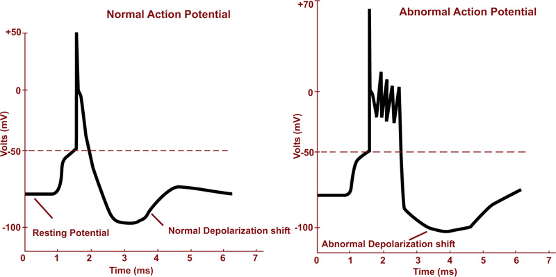
Seizure is an irregular neural activity in the form of a sudden uncontrolled electrical discharge in the cortical brain region. As a result, a collection of nerve cells starts firing excessively and synchronously. People with frequent and unprovoked seizures, are usually diagnosed as epileptics [17, 34]. The action potentials in normal and during seizure activity are depicted in Fig. (2a).
2.2. ECoG Signal
Generally, EEG records can be made non-invasively from the scalp or invasively via surgical implantation of invasive electrodes in the intracranial structures. The Intracranial EEG (iEEG) consisting of electrocorticography (ECoG) or stereotactic EEG (sEEG) is the neuroelectrophysiologic signal acquired from implanted subdural or depth electrodes, respectively [35, 36].
Scalp EEG recordings are limited by the extracranial artifacts caused by the scalp muscle and heart activities, eye movement, external electromagnetic field, etc. Therefore, removing the artifacts from EEG signal stays a key challenge for finding valuable information from brain activities [37, 38].
As an invasive method, iEEG recording presents a higher signal-to-noise ratio (SNR) compared to scalp EEG [10, 13, 39, 40]. The invasive electrode is able to record signals from the small-population neurons, which is non-recordable with the scalp one. Once the intracranial EEG is employed to record the brain activity, the brain wave is not weakened or changed by the skull/scalp tissue, which performs like a low-pass filter. Then, the seizures can be identified typically earlier employing the intracranial electrodes compared to the scalp electrodes [41-44].
2.3. SOP and SPH Definitions in Seizure Forecasting
Let us introduce three important time intervals in the field of seizure forecasting:
- Seizure occurrence period (SOP), the time interval in which a seizure is expected to occur [10, 45, 46].
- Preictal period (PP) or preictal zone, the period before a seizure, which is clinically obscure but implicitly determined in the dataset [47].
- Seizure prediction horizon (SPH), the interval between the alarm and a leading seizure expected to occur. This period is also vague though it should be in the preictal period [10, 45, 46].
During the SPH interval, a seizure-warning tool can effectively inform the patient to behave carefully or treatment plans can be employed [45]. Based on the clinical aspect, SPH should be high enough to allow sufficient time for the patient to behave cautiously or take medicines. By contrast, SOP should be low enough to soothe the patient’s anxiety and stress [45, 46].
2.4. The Challenges of Seizure Anticipation
During the past quarter century, there has been an acceleration in the development of novel medical devices, from which implantable medical devices (IMDs) have been gaining increasing interest for biomedical applications including physical identification, health diagnosis, monitoring, recording, and treatment of the physiological characteristics of the human body [48-50]. Despite a great deal of research in seizure prediction, an accurate and cost-effective seizure forecasting system remains elusive [9]. The capability of machine learning (ML) algorithms in producing very accurate results has influenced scholars to solve various challenges of real-world problems by recruiting ML techniques, with several researchers proposing ML-based algorithms for predicting an epileptic seizure in the last few years [2]. Let us review some of the key challenges in implementing of future IMDs in the prediction of a seizure.
2.4.1. Nonstationary Nature of the Brain Activity
In order to diagnose a brain disorder, one may need first to decode the brain activity. The brain, the most complex structure present in the human body, contains more than 100 billion neurons [51-53] with hundreds of trillion nerve connections that form the neural circuits [51, 52]. These circuits can be involved in numerous brain activities and functions via engaging multiple neurons. This is further complicated because neurons have multiple functions and neurons communicate with one another [21, 52, 54]. Then the EEG signal measures the field potentials of many neurons and theoretically, the activity of neuronal assemblies (considered as a non-linear dynamical system) should undeniably involve non-stationary and non-linear time-dependent functions [2, 55-57]. Furthermore, the uncertainty of the brain signals is highly susceptible to various forms and sources of noise and may diligently resemble an impending seizure. Consequently, employing other biological measures like heart rate variability, blood pressure, photoplethysmography (PPG), and electrodermal activity (EDA) have been shown to enhance forecasting performance [8, 57].
2.4.2. Low- Power Implantable Medical Device (IMD)
There are various challenges in designing of IMDs such as size, power consumption, biocompatibility, reliability, and lifetime [48, 49, 58]. Power consumption perhaps plays a dominant role among others and even can have effects on other factors [58]. As the size of the IMDs is continuously decreasing, the need for developing a reliable data processing technique that is computationally efficient for implementation on hardware is tremendously demanding [9, 59, 60]. Also, running complicated algorithms on the IMDs requires a large physical size, which requires excessive power dissipation. Moreover, high-power consumption and losses generate unavoidable heat and consequently the temperature around the body organs will rise, which grow the possibility of body rejection and the likelihood of developing cancer and even downgrading the longevity of implantable biomedical devices [58].
On the other hand, some of the recently developed algorithms are computationally expensive and demand additional resources to achieve high reliability so an optimal design is required to intelligently compromise the power dissipation and the performance metrics [9]. In (Table 1), a summary of the power requirement of several IMDs is reported [9, 58, 61].
2.4.3. Related Works
Research on seizure prediction via an electroencephalograph (EEG) recording started in the 1960s [62]. Since then, many techniques have been developed but there is still room to enhance the performance of the prediction results. A review of the studies related to this research is summarized in Tables 2 and 3. In these works, accuracy was, most of the time, considered as the plain performance measure while the window size has been also investigated.
The authors employed accuracy on a highly imbalanced dataset to find the best window size, i.e., 20 s, from a set of 1 to 60 s window lengths [10]. However, accuracy alone cannot be considered the best metric to use and the results of this work need to be re-evaluated by applying other measures besides accuracy. In fact, in the above work, very few pre-ictal samples were studied, while most of the samples belonged to the inter-ictal segments. Then, the model may gradually lose its capability of predicting the preictal patterns succeeding a long inter-ictal pattern. Same conclusion can be made on the work discussed in [63]. On the same framework, Parvez [25] claimed that a 10 s window outperformed due to being more consistent with respect to the AECR (Average Energy Concentration Ratio) values of preictal and interictal segments, although the length of the data in this experiment was about 10 minutes. Then the above statement needs to be reinvestigated as well for a larger set of data.
Sigh employed the posterior probability of the classifier and compared it for various window sizes and then, the 90 s window was chosen due to having the highest posterior probability while the performance of the model was not reported and whether under-fitting or over-fitting were resolved during the training or not [64]. Some authors calculated the correlation coefficient during a certain time window (from 0.5 to 300 seconds) and investigated the performance of the classifier just by employing AUC [28]. They found out that the time window of 60 s and 30 s demonstrated the highest AUC for seizure prediction in humans and dogs, respectively. Again, the imbalanced data ratio was not reported, while AUC demonstrated various flaws and drawbacks owing to the fact that it is sensitive to class imbalance [65-67].
With regard to Table 3 [10, 68, 69], the classifiers were optimized based, again, on one measure, i.e., accuracy. Furthermore, the performance of the classifier was not reported [47] and it was based on other parameters rather than accuracy. From the above, we can see that the major disadvantage of the above studies in finding the optimum window length is using plain accuracy, which can be an inadequate metric to evaluate the performance of the classifier [70-73], particularly while dealing with imbalanced data, as in most of the existing databases.
| Reference, year | Feature Used | Window Size Used in the Paper | # of Subjects and Seizures | Performance of the Classifier | Imbalance Ratio (Data Length) |
| [10], 2018 | Area, Normalized decay, Line length, Mean energy, Peak amplitude, Valley amplitude, Normalized peak number, Peak variation | 1-100 s | 7 subjects (5 dogs and 2 humans) | Accuracy | 20:1 for dogs 2:1 for patients |
| [64], 2016 | Power Spectral Entropy,
Fast furrier Transform, Higuchi Fractal Dimension, and Hurst Exponent |
10-600 s | Optimal window size can be argued to be around 90 seconds | ||
| [28], 2015 | Calculate the correlation coefficient in a
Certain time window between all possible pairs of EEG signals |
0.5-300 s | Kaggle dataset, 5 epileptic dogs and 2 epileptic patients | AUC, no other information about the classifier performance | In humans, best classification is showed by SVM classifier for a time window Tw = 60 s (AUC = 0.9349); for seizure prediction in dogs, highest obtained AUC is 0.9432 for SVM classifier and Tw = 30 s |
| [63], 2008 | Empirical Mode Decomposition (EMD) and AR model coefficients | 12, 24, 35, and 47 s | 19 patients
the Freiburg database |
Accuracy and variance | From 5 to 20 min of preictal and same length from interictal |
| [25], 2016 | Average of the energy concentration ratio | 5, 10, 15 seconds | 21 patients | No information | 10 second window outperformed due to being more consistent with respect to the AECR values |
| Reference, Year | Avg. Pediction Time | Feature Used | Performance Analyzing & Classifier’s Performance | Imbalance Ratio (Data Length) | Database (Patients, Human/Dog) | # Seizures and # Hours Data |
| [68], 2019 | 0.25 minutes | Nonlinear features (which are computationally expensive) | sensitivity of 91% FP:36% | -- | 16 patients / Boston Hospital non-invasive EEG | The number of seizures is not mentioned Less than 60 hours data were investigated |
| [10], 2018 | Not reported | time and frequency domain | FP/h=0.03-0.6 TP/h=40-97% For human: TP/H:0.4-0.74 FP/H: 0.26-0.6 & Accuracy |
From 2:1 to 20:1 677 hours (42 hours for human) 111 seizures (10 for humans) |
MSEL-LAB 7 subjects (5 dogs and 2 humans) |
MSEL and IEEG.ORG |
| [47], 2017 | No information provided | time and frequency domain | Prediction can achieve a sensitivity of about 90–100%, and the false-positive rate of about 0–0.3 times per day. No performance classification is reported. |
8:1 to 10:1 (607:77) |
Kaggle competition (6 Dogs) canine epilepsy is an excellent analog for human epilepsy |
20 seizures |
| [69], 2017 | 33 | time and frequency domain | Sensitivity=92.2%, and specificity 93.38%. or 0.06 1/h & accuracy |
Not mentioned | CHB-MIT, scalp | 84 seizures, 22 subjects |
| [74], 2017 | 25.66 | 26 univariate and 3 bivariate features | Sensitivity79% Specificity 82% |
Not mentioned | 10 patients 26 electrode iEEG |
154 seizures 86.20 days data |
| Patient# | Sex | Age | Seizure type | H/NC | Origin | Electrodes | Seizures analyzed |
| 2 | M | 38 | SP, CP, GTC | H | Temporal | d | 3 |
| 4 | F | 26 | SP, CP, GTC | H | Temporal | d, g, s | 5 |
| 7 | F | 42 | SP, CP, GTC | H | Temporal | d | 3 |
| 10 | M | 47 | SP, CP, GTC | H | Temporal | d | 5 |
| 12 | F | 42 | SP, CP, GTC | H | Temporal | d, g, s | 4 |
| 16 | F | 50 | SP,CP, GTC | H | Temporal | d, s | 5 |
3. MATERIALS AND METHODS
3.1. Dataset
The EEG dataset employed in this research is from the University Hospital of Freiburg, Germany. The Freiburg EEG Database (FSPEEG) is one of the most cited resources employed in predicting and detecting experiments. The EEG-database consists of two sets of files: “preictal (pre-seizure) data,” i.e., epileptic seizures with up to 120 min preictal data, and “interictal data,” which contains about 24 hours seizure-free EEG-recordings [75]. The EEG-database comprises six intracerebral (strip, grid, and depth electrodes) EEG recordings with a sampling rate of 256 Hz. We retained six epilepsy patients (temporal lobe epilepsy with the hippocampal origins (134 hours) from this set of data (mean age: 31; age range: 14-50; both gender) and employed 50 seizures in this study from these 6 patients (Table 4).
3.2. Methodology
3.2.1. Preprocessing and Feature Extraction
The initial step in iEEG signal analysis is preprocessing. To reduce the impact of factors that cause baseline differences among the different recordings within the dataset and eliminate the signal DC component, iEEG signals were standardized using Z-scores (expressed in terms of standard deviations from their means). The only potential artifact that could be addressed was the harmonic power line interference at 50 Hz. We eliminated the 50 Hz interference indirectly by performing sub-band filtering. So, preceding feature extraction, we used six band-pass FIR (Finite Impulse Response) filters to split the iEEG signals into various frequency bands: Delta (0.5-4 Hz), Theta (4-8 Hz), Alpha (8-12 Hz), Beta (12-30 Hz), as well as two Gamma bands namely, low-Gamma (30-47 Hz), and high-Gamma (53-120 Hz) [76-78]. This led to an input space of 306 dimensions per window.
To handle the unbalanced data set, an hour EEG signal was split into several non-overlapping window sizes (from 1 to 40 seconds) for the interictal stage, whereas the preictal stage was divided into chunks of the same window sizes with 50% overlapping. Although the time-frequency domain features are most informative, the time-domain ones are more appropriate to attain discriminative information at a low computational cost. In fact, high-quality features can be defined as those that generate maximum class separability, robustness, and less computational complexity, e.g., less complex preprocessing that does not need the burdensome task of framing, filtering, Fourier transform, and so forth [23]. Thus, these features, compared to other types, consume less processing power and time. Consequently, from the three above-mentioned domains, we retained the features that belong to the time domain. Several univariate linear measures were extracted at each epoch of window length, along with a bivariate linear measure, as reported in Table 5 [79-81]. From this table, we can conclude that the proposed system can work in real-time; in fact, the features can be computed and the classifier can deliver an output in less than the window length. More details about such time domain features can be found in another work [82].
| S. NO. | Features | Comments | Time of the Computation for Each Channel (s) |
| 1 | Interquartile range | One feature (36D)1 | 0.036152 |
| 2 | Mean Absolute Deviation | One feature (36D) | 0.010459 |
| 3 | Hjorth complexity | One feature (36D) | 0.003935 |
| 4 | Coefficient of Variation | One feature (36D) | 0.010528 |
| 5 | MAX of cross correlation | 15 values for 6 channels, but considered as one feature (90D) | 0.087968 (between two channels) |
| 6 | AR model 2 | Two features (72 D) | 0.026372 |
3.2.2. Data Partitioning
We used two approaches for validation namely, ‘Hold-out’ and ‘k-fold cross-validation’.
3.2.2.1. Hold-Out
In the hold-out validation, we considered 75% of the data for learning (training) and the remaining 25% for final evaluation (testing).
3.2.2.2. K-Fold Cross-Validation
To apply ‘k-fold cross-validation’, the dataset is first divided into ‘k’ folds. Each time, only one fold is employed for testing and the others are employed for training the model. Then, the model is trained on the training subset and evaluated by the validating subset. This process is repeated until each distinct fold is used as a validation subset. For this study, we employed 10-fold cross-validation and ran each cross-validation experiment 10 times, i.e., 100 runs for each model. Finally, the average of the obtained set of accuracy values was considered [83-85].
In a nutshell, we split the data into two groups, train set (which consists of 75% of the data for tuning and validating the model) and the remaining data as the test set (never-seen-before). Both training and testing data segments have been numbered sequentially [86, 87]. When the classifier was fully optimized with the learning and validating subsets, via 10-fold cross-validation, it was applied to the test set for final evaluation of the selected model.
Undeniably, our aim is to prevent overfitting and underfitting and provide a generalized model that can make an accurate prediction on future unseen data. Overall, we examined the predictive power of unknown data and provided an unbiased estimate for the predictive performance of the model [87-89].
3.2.3. Classification Approach
In this work, we used different classification approaches such as Support Vector Machine (SVM), Multilayer Perceptron (MLP), Random Forest (RF), and XGBoost (XGB).
Support Vector Machine (SVM) is one of the most popular machine learning methods for classification. SVM utilizes the loss function, hinge, to find the optimal regularization parameter, C. We employed linear SVM with L1 regularization to struggle with overfitting so that the model can produce well to predict new data. L1 regularization is the suitable choice for built-in feature selection and when the output is sparse [90, 91].
MLP is a feed-forward Artificial Neural Network (ANN). We retained the Relu function as nonlinear function employed in the hidden unit and tuned alpha as the regularization parameter [20, 90, 91].
Random Forest is one of the most effective methods in machine learning, consisting of creating models so-called as ensemble [88]. After training, the model tries to predict every tree in the forest, then combines individual predictions based on a weighted vote. This means that each tree gives a probability for each possible target class label, then the probability for each class is averaged across all the trees and the class with the highest probability is the final predicted class [92]. We tuned the maximum depth for the tree to regulate the complexity and decrease overfitting [89].
XGBoost stands for eXtreme Gradient Boosting, the fast implementation of gradient boosting. Boosting is a sequential ensemble learning method to adapt a series of weak base learners to strong learners to increase the performance of the model [89, 93-97]. XGBoost involves a much faster computation than the regular gradient boosting algorithms since it employs parallel processing. To enhance the model, the XGBoost classifier has two regularization terms (inbuilt L1 and L2) to penalize the complexity of the model and avoid overfitting [56, 93, 97].
We used the scikit-learn (machine learning) library through the python package for this work [98]. The experiments were executed on a desktop computer with Intel® Core™ i7 CPU @ 3.3 GHz processor, 16 GB RAM, and Windows 7 Professional 64-bit operating system.
3.2.4. Evaluation and Performance Analysis
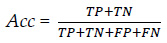
A classifier must generalize, i.e., it should work well when submitted to data outside the train set. As we are handling the issue of imbalance distribution of data, accuracy cannot be an adequate metric to evaluate the performance of the model [70-73]. While accuracy remains the most intuitive performance measure, it is simply a ratio of correctly predicted observations over the total observations, so reliable only when a dataset is balanced. However, this measure has been utilized exclusively by some researchers in analyzing seizures [10, 99, 100].
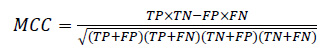
Various metrics have been developed to evaluate the effectiveness and efficiency of related models in handling imbalanced datasets such as F1 score, Cohen’s kappa, and Matthews’s correlation coefficient (MCC) [68-70]. Among the above popular metrics, MCC can be seen as a robust and reliable evaluation metric in the binary classification tasks and, in addition, it was claimed that measures like F1 score and Cohen’s kappa should be avoided owing to the over-optimism results, particularly on imbalanced data [71, 72, 101, 102].
The confusion matrix has been utilized to visualize and evaluate the performance of a classifier (Table 6). After computation, we utilized accuracy and MCC to compare the classification performance and effectiveness of the feature selection methods. Hence, we categorized iEEG data into two classes: “1” denoting the pre-ictal stage and the period prior a seizure and “0” denoting seizure-free periods (interictal) and postictal (the period of time after a seizure).
| Actual | Predicted | |
| Positive | Negative | |
| Positive | TP (True Positive) | FN (False Negative) |
| Negative | FP (False positive) | TN (True Negative) |
3.2.4.1. Accuracy (Acc):
Accuracy can be described as the ratio between the number of correct predictions and the total number of correct predictions. Let TP be actual positives that are correctly predicted positives, TN be actual negatives that are correctly predicted negatives, FP actual negatives that are incorrectly predicted positives, and FN actual positives that are incorrectly predicted negatives. Therefore, accuracy can be stated as:
 |
(1) |
3.2.4.2. Matthews’s Correlation Coefficient (MCC):
MCC ponders all four quadrants of the confusion matrix, which gives a better evaluation of the performance of classification algorithms. The MCC can be considered as a discretization of Pearson’s correlation coefficient for two random variables due to taking a possible value in the interval between -1 and 1 [102-104]. A score of 1 is supposed to be a complete agreement, −1 a perfect misclassification, and 0 indicates that the prediction is no better than random guessing (or the expected value is based on the flipping of a fair coin).
 |
(2) |
3.3. Optimum Window Size
As mentioned above, an iEEG signal was chunked into various segments and during each sliding window, a specific feature was extracted. This is repeated until the whole signal is treated. The time window size varies from study to study from 1 to 20 seconds [10, 45-47, 105] and some work have been done about finding an optimum length of seizure prediction [25, 64, 106]. However, due to a lack of information related to the performance of the classifier, this issue still needs further investigation.
The length of the window is a crucial parameter that needs to be chosen carefully. This size cannot be deemed too small since the signal requires to be long enough to provide reliable values for the features. Furthermore, the aim of this work is to implement an algorithm on a low power device, which usually means limited computing power. Then with very small window size, less computational power is required to compute in each window compared to the longer one. This can pose a threat once enough computational power could not be available on a small implantable medical device [100, 106]. On the other hand, the window size cannot be taken too long because the characteristics extracted from the signal will not have a very smooth transition over time. In fact, because the targeted activity might occur at the beginning or in the middle of the window, the values extracted for the whole part of the sliding long-window may not exactly represent the type of activity [100].
The outputs of the classifiers for different sets of window lengths, depicted in Fig. (3), highlight MCC score as the highest for the XGBoost classifier, while MLP demonstrated the least performance. From Table 7, one can notice that SVM requires the lowest time and memory for the classification process. However, XBG being the most time-consuming approach due to implementing an ensemble boosting approach that converts various weak learners into complex model sequentially, the final criterion to choose the best classifier was the performance metric, MCC.
Among the available classifier candidates discussed above, XGBoost gave the best performance in binary classification with the highest MCC score while the grid search was performed to optimize the Maximum depth parameter. XGB has been broadly utilized in numerous fields to demonstrate state-of-the-art results on some data challenges and it has shown a strong potential to solve the resulting difficulties in data analysis. Besides, it is one of the most favorable classifiers in machine learning regarding classifiers [95, 107, 108].
| Time and Memory for each classifier | XGB | RF | MLP | SVM |
| Elapsed CPU-Time (s) | 2.11 | 0.75 | 0.79 | 0.27 |
| Memory consumption (kB) | 2.79 | 157.03 | 19.61 | 0.5 |
Finally, MCC score of XGB for various window sizes was displayed in Fig. (3), showing that the best MCC was located in the range of 2-10s window.
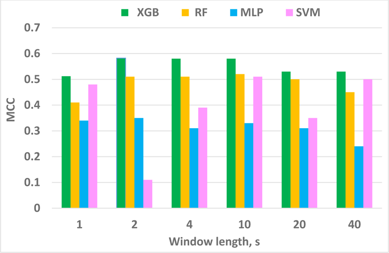
Note that our work does not suffer from the imbalanced issue, which ratio is 1.6 (52 and 82 hours preictal and interictal, respectively). Various performance measures and classifiers were applied to make sure the prediction system was investigated thoroughly. For a window length of 1 s, the classifier performance was not improved, which can confirm Islam’s works [29, 109] that state that by selecting a very short window, e.g., less than one second, the seizure waveform may not be recognized properly in such a short duration. On the other hand, by considering a longer window length, e.g., more than 3 seconds, the assumption of stationarity of an EEG signal is not valid anymore. Hence, artifacts and seizures cannot be distinguished from each other.
In a nutshell, a non-stationary signal like EEG can be assumed as a stationary signal in a short duration epoch like a 2-second window. Another point to note is that, in order to optimize the device performance for a real time processing, one needs to take into consideration the factors of computing resources, power consumption and CPU time in a real time processing. In a real time scenario, a device will be always sequentially extracting and calculating some features. Then by assuming a longer window size, the device will need to calculate the features based on a longer portion of the signal. The longer the window size, the higher will be the power consumption and CPU time.
3.4. Probabilistic Framework
In order to undertake this research, various phases were recruited: data collection, data preprocessing and feature extraction, classification and optimization, evaluation and decision-making (which will be discussed later). The overview of the proposed pipeline is illustrated in Fig. (4).
3.4.1. Platt Scaling
Platt scaling is used to extract the probabilities of each class, i.e., seizure vs. non-seizure. This calibration method passes the output of a classifier from a single model to a probability distribution through a sigmoid, as a result estimation of posterior probability in 0-1 range [110, 111].
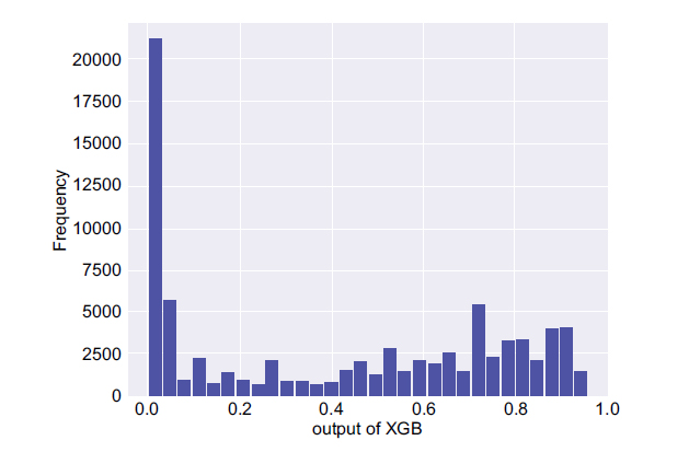
In the next step, two important parameters were calculated, namely, the mean and maximum probability of the non-seizure (PNS) and the seizure occurrence period (PSOP) segments for each participant along with the maximum probability of the PIN. The histogram of Platt scaling for the whole test set (PIN) is illustrated in Fig. (5). It shows that the model predicts most of the time the lowest value and the chance of having a seizure is not too high. However, in the case the system creates a very high probability value then, possibly, one should have been dealing with a high rate of false positive rate since a large set of interictal section had been employed.
3.4.2. Thresholding
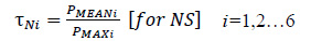
Success in learning the data using the optimized XGBoost framework and extracting the probabilities as described earlier, few adaptable thresholds were chosen to forecast the seizure efficiently based on the following procedure. In order to set the thresholds (τN, τS) for 6 patients, the average and the maximum probability of non-seizure (NS), the seizure occurrence period (SOP), and the maximum probability of PIN (PMAX) were computed. Then τN and τS were defined as follows:
 |
(3) |
 |
(4) |
These empirical constants were considered as thresholds based on numerous experiments for the 6 patients and then, in order to predict an impending incident, a simple model was then retained.
3.4.3. Decision Making
The pseudo-code of the supervised prediction framework for an impending incident can be described as follow:
1: procedure PREDICTION (PIN, τN, τS,PMAX,POUT)
2: input: PIN, τNi, τSi,PMAXi (i=1, 2,…, 6)
3: output: POUT
4: for each time point of PIN
5: if PIN ≥ PMAXi then
6: go to line 11
7: else if PMAXi > PIN ≥ MEAN (τNi and τSi) then
8: return activate PA1(Prediction Alarm level 1 during T1)
9: P1 ← compute average of PIN over a 1-minute window
10: if P1 > MAX (τNi /τSi and (τNi + τSi)/2) then
11: return trigger PA2 (Prediction Alarm level 2 during T2)
12: else go to line 7
13: end if
14: else go to line 5
15: end if
16: end for
17: end procedure
As shown in this algorithm, the probabilistic prediction framework sequentially employs a 270 dimensional feature-set (extracted 6 features over a 2-s window) to generate PIN as one of the inputs to the probabilistic prediction framework (along with τNi, τSi, and PMAX). Based on the PIN value and the first set of thresholds (τNi, τSi), the system triggers the first prediction alarm (PA1) to warn the patient of an upcoming seizure with about 60% probability (the average of τN and τS) within the period T1. If PIN is higher than PMAX, then a second alarm (PA2 as T2) will instantly be activated. Afterwards, the function accumulates the input for one minute (the future window length can be called the forecast horizon) to generate the second level of warning. This is done with the succeeding set of thresholds (MAX of [τNi /τSi and (τNi + τSi)/2]), which entrust 80% for an impending seizure (PA2) at a certain time T. Finally, it sends an urgent alert to the patient and caretaker. Interestingly, in most published works, the anticipation time of the first alarm has been reported while in this work, we provided two sets of alarms to finally compare our work with others based on the first triggered alarm.
If the second condition is not met, at least the primary flag is raised and the system will continue to accumulate the next minute PIN to satisfy the PA2 condition. This procedure will continue as PIN ≥ (τNi +τSi)/2 and up to T2 times (i.e., this procedure will continue, T2 will be updated, and the system will remain active to make sure the seizure will happen as predicted earlier). The whole procedure is repeated until the end of the iEEG signal (Table 8).
4. RESULTS AND DISCUSSION
4.1. Evaluation of the Probabilistic Approach
After optimizing a classifier, the performance of the overall prediction was measured using common metrics utilized in the field to verify and estimate how successfully the proposed algorithm performs. Sensitivity of the triggered alarms and false prediction rate (FPR) were employed to demonstrate the results of this research and compare them with related works. Sensitivity measures the ratio of correctly predicted seizures divided by the total number of seizures, while the false prediction rate (FPR) is the number of false predictions over the total number of negatives [112].
 |
(5) |
Since in this work it is critical not to miss the seizure events (preictal), the aim was to maximize the sensitivity or True Positive Rate (TPR) [113] and, at the same time, to have a low FPR. Conventionally, in order to set a threshold, some researches plotted the TPR vs. FPR (the ROC curve). So, in order to maximize the performance of the prediction, there is a trade-off to find the best threshold between avoiding a great number of false positives (FP) and benefiting from true positive (TP). In fact, it is challenging to simultaneously lower the number of false alerts and increase the sensitivity [107, 113-115]. In the last decade, various approaches have been employed by scientists to attain an increase in the sensitivity and a decrease of the low False-Positive rate while targeting a high anticipation time [45, 64, 115, 116]. If the outcome is above the threshold, a seizure alarm is triggered (in this work the values of the alarm were inserted in the first stage). As explained earlier, the threshold values of our seizure prediction framework are set so that they do not miss seizure episodes.
4.2. Results and Comparison with other Works
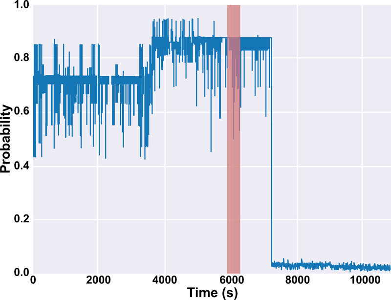
The results of this work for both sets of alarms are depicted in Table 9 and 10. It is mentioned in Table 9 that there are two values of T for patients #10 and #16 since we tested the model on two seizures for those patients. Also, the output of the probabilistic model based on Platt scaling (PIN in Fig. (5) for patients #10 and #12 were illustrated in Figs. (6 and 7), respectively. In Fig. (6), PIN for both preictal and interictal segments was demonstrated. The seizure is happening between 5980 s and 6133 s (highlighted in red) before the interictal sections. The seizure period is highlighted in red for patient #12 in Fig. (7). The proposed prediction system is not only capable of forecasting the seizures (high sensitivity) but also will not generate a high false alarm (Table 10).
| Pa#2 | Pa#4 | Pa#7 | Pa#10 | Pa#12 | Pa#16 | The average with 95% confidence interval | ||
| PNS | PMEAN PMAX τN = PMEAN/PMAX |
0.2068 0.53349 0.387717 |
0.002508 0.01957 0.12815 |
0.06607 0.3059 0.21597 |
0.02169 0.05004 0.43337 |
0.00249 0.0233 0.1069 |
0.0194 0.03959 0.49087 |
0.0532 0.16198 |
| PSOP | PMEAN PMAX τs = PMEAN/PMAX |
0.34057 0.4499 0.75699 |
0.0644 0.10319 0.62446 |
0.16109 0.3059 0.5266 |
0.7457 0.9039 0.8251 |
0.76478 0.8478 0.902 |
0.623 0.863 0.7219 |
0.44997 0.57899 |
| (τN+ τS)/2 τN / τS MAX([τN+ τS]/2 & τN /τS) |
0.572 0.51218 0.572 |
0.3763 0.2052 0.3763 |
0.3713 0.41013 0.41013 |
0.6292 0.52527 0.6292 |
0.5045 0.11849 0.5045 |
0.6065 0.6799 0.6799 |
0.51 0.41 0.53 |
|
| Maximum probability of PIN, (PMAX) | 0.6435 | 0.59142 | 0.7376 | 0.94712 | 0.9173 | 0.9577 | 0.7991± 0.09 | |
| Time of prediction | Pa#2 | Pa#4 | Pa#7 | Pa#10 | Pa#12 | Pa#16 | The average with 95% confidence interval |
| for PA1, T1 (min.) | 59.6 | 70.2 | 68.4 | 88.7 & 80.3 | 85.1 | 67.1 & 84.9 | 75.5±7 |
| for PA2, T2 (min.) | 55.9 | 70.1 | 43 | 82.7 & 38.8 | 55.6 | 15.6 & 33.1 | 49.4±14 |
| Results | Average for all the patients based on PA1, T1 | Average for all the patients based on PA2, T2 |
| Sensitivity | 100% | 100% |
| FPR | 0.07% | Almost 0% |
| Anticipation Time | 75.5±7 | 49.4±14 |

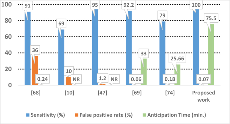
As demonstrated, the proposed approach performs better with the highest sensitivity and the lowest false positive rate (Fig. 8). As mentioned earlier, our comparison is based on the first set of alarm, PA1, and the anticipation time is considered T1. It is worth mentioning that these results should be relativized because of the limited number of patients available in the used database.
CONCLUSION
In this work, an efficient probabilistic seizure prediction tool was proposed. Based on the XGBOOST algorithm, it uses a novel threshold method to predict the seizure with an invasive approach. With a sensitivity and specificity of almost 100%, the anticipation time can be up to about 75 minutes, a period long enough to provide adequate clinical treatment time prior to a seizure. Furthermore, the proposed algorithm does not rely just on an early warning since the medical decision-making continues to inform the patient for the upcoming seizure, making it an efficient tool for significantly improving the daily life of patients.
LIST OF ABBREVIATIONS
| iEEG | = Intracranial Electroencephalogram |
| DBS | = Deep Brain Stimulator |
| VNS | = Vagus Nerve Stimulator |
| AED | = AntiEpileptic Drugs |
AUTHORS' CONTRIBUTIONS
Software, B.A.; visualization, B.A.; writing—original draft preparation, B.A.; writing—review and editing, B.A., C.T., and M.C.E.Y.; supervision, C.T. and M.C.E.Y. All authors have read and agreed to the published version of the manuscript.
ETHICAL STATEMENTS
The retrospective evaluation of the data received prior approval by the Ethics Committee, Medical Faculty, and University of Freiburg.
CONSENT FOR PUBLICATION
Informed consent was obtained from all subjects involved in the study.
STANDARDS OF REPORTING
STROBE guidelines were followed.
AVAILABILITY OF DATA AND MATERIALS
The data is freely available on the internet at https://epilepsy.uni-freiburg.de/freiburg-seizure-prediction-project/eeg-database.
FUNDING
None.
CONFLICT OF INTEREST
The authors declare no conflicts of interest, financial or otherwise.
ACKNOWLEDGEMENTS
Declared none.