All published articles of this journal are available on ScienceDirect.

Implantable Device Positioning based on Magnetic Field Detection using Genetic Algorithm in Body Area Biosensor Networks
Abstract
Background:
Minimally invasive medical care by the aid of Information Communication Technology (ICT) has attracted considerable attention. Sensor nodes including implantable devices within the bio-sensor network or Body Area Network (BAN) have been utilized to reduce the burden on patients. To control the operation of devices properly or collect vital data effectively, it is important to obtain accurate information on their position.
Methods:
This paper provides an effective positioning method based on the detection of magnetic fields generated from implantable devices using the Genetic Algorithm (GA). After providing the principle of the proposed method, some laboratory test measurement results are given to confirm its effectiveness.
Results:
Magnetic field detection using multiple magnetic field sensors was achieved. From the results of multiple point measurements on the three-dimensional components of the magnetic field strength, the position of the target was obtained with a smaller error. Laboratory test measurement results are in good agreement with the theoretical values.
Conclusion:
The proposed positioning method is an effective and an economical approach. It is also effective for detecting moving devices such as a capsule endoscope in a human body. With the aid of the GA, high-speed detection is obtained with a low calculation costs. The compressed sensing method reduces the number of measurement points.
1. INTRODUCTION
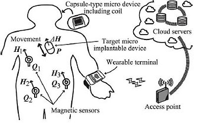
To realize short range communications, Wireless Body Area Networks (WBANs) and sensor networks have attracted considerable attention for their use in the Internet of Things (IoT) [1-5]. Above all, biosensor networks supported by Information and Communication Technology (ICT) as shown in Fig. (1) play an important role in medicine, point-of-care and health care, and so forth. To realize effective biosensor networks including implantable devices such as capsule endosco-pes as sensor nodes, it is important to obtain effective control and communication methods. To accomplish these objectives, it is necessary to develop an accurate positioning method and an efficient signal transmission method. In this case, we should detect devices in the human body accurately from outside.
With regard to the positioning method, we can detect the positions of devices with multiple installed antennas [6] when wireless communication technologies such as Bluetooth are introduced [7]. A detection method using electromagnetic waves has been previously reported [6]. To minimize the burden on the human body, the magnetic field detection is preferable to the electric field detection of radio waves. The adoption of a Superconducting Quantum Interference Device (SQUID) sensor used for Magnetoencephalography (MEG) in medical engineering can provide an accurate positioning method under a small magnetic field of 10-15 to 10-13 T [8, 9]. However, particularly in the latter method, the system is expensive and requires the installation of complex equipment. In addition, it is difficult to ensure good wireless communication during the positioning process because of the interference due to the strong magnetic field around the human body. Therefore, a safe and economical positioning method with high accuracy is required. Mobility support is also required for future biomedicine applications, although few studies have so far been carried out on this matter [10].
With the above motivation, we propose an effective positioning method under limited battery power operation. The proposed method has a low cost and is based on the magnetic field detection of implantable devices including capsule endoscopes. The rest of this paper is organized as follows. In Sec. 2, related works are described. In Sec. 3, we introduce the principle of the proposed method. Then, in Sec. 4, a theoretical analysis of the proposed method is given. In Sec. 5, some laboratory experimental results are provided to show the effectiveness of our proposed method. The final section summarizes the paper.
2. RELATED WORKS
As mentioned in Sec. 1, implantable device positioning can be performed electrically or magnetically [6-10]. From the viewpoint of non-invasive measurement and independence of the permeability of the human body, a magnetic approach is preferable. In this case, precise detection in a short period by an economical method is needed. By measuring the magnetic field strength, we can perform positioning by solving the high- order nonlinear simultaneous equations as shown later. Thus, considerable labor is required to obtain the position of the target. To avoid complicated calculations, a simple mathematical method of solving high-order equations as a reverse problem is given in [11]. Instead of solving high-order equations, the adoption of Artificial Intelligence (AI) is an effective option for obtaining a good solution based on multiple measurement data of a magnetic field.
Regarding the positioning methods used in healthcare, in [11], the positioning methods based on magnetic fields including Radio-Frequency (RF) positioning [12-14] were surveyed. It was stated that the optimal choice depends on the specific field of application. However, these methods are not for implantable devices but for human motion. Moreover, the adoption of AI was not mentioned. On the other hand, in the field of healthcare, there are many papers dealing with AI [15-17], showing its effectiveness as a method of determining the optimum solution of problems. Thus, to achieve our objectives, we also apply an AI-based method.
3. PRINCIPLE OF PROPOSED METHOD
3.1. Detection of Superimposed Magnetic Field
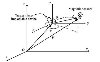
The concept of proposed positioning method is depicted in Fig. (2). It is assumed that the measurement target is at the point P(xp, yp, zp) in three-dimensional (3-D) space. Owing to mobility of the target, it moves with a nonzero velocity. However, without loss of generality, we consider that the target is fixed at one position. We measure the magnetic field strength using multiple magnetic field sensors located at arbitrary points Qi(xi, yi, zi) (i = 1, 2,···) around the target. When the target implantable device operates with the consumption of electric power, an additional magnetic field, ΔHi,(i = 1, 2, ...) will be superimposed on the geomagnetism component H0 i(i = 1, 2, ...). Thus the total magnetic field at point Qi(i = 1, 2, ...), Hi, can be given as Hi = H0 i + ΔHi (i = 1, 2, ...). Here, bold variables indicate vectors. H0 i and ΔHi satisfy the inequality |H0 i| >> |ΔHi|. |H0 i| is about 2.4 × 10⁻⁵ to 6.6 × 10⁻⁵ T, whereas |ΔHi| is less than 1 × 10⁻⁷ T owing to the low power consumption within an electronic circuit. When we consider the 3-D magnetic field components at the measurement point, the background geomagnetic components H0 i are equivalent to each other. This is because the distance among the magnetic field sensors are sufficiently small (less than several ten inches) to have significantly different values. On the other hand, the superimposed components are different. From the 3-D magnetic field vector at each point, Hi (i = 1, 2, ...), we can calculate the position of the device. This calculation requires the solution of an inverse problem. Note that the sensitivity of the magnetic field sensors must be sufficiently high to detect the superim-posed components. To meet this requirement we can use magnetoimpedance (MI)-type sensors [18, 19]. A typical sensitivity of an MI-type sensor is 1 V/μT [20].
3.2. Magnetic Dipole
It is convenient to introduce a 3-D global coordinate system and a local coordinate system when we deal with mobile implantable devices. As shown in Fig. (2), it is assumed that a magnetic dipole is located at point P in the global coordinate system, which corresponds to the origin of the local coordinate system. The following discussion is based on the local coordinate system unless otherwise stated. We assume that the measurement point is Qi (Ri, Θi, Φ i) in spherical global coordinates, where Ri is the radial distance, Θi is the polar angle, and Φi is the azimuthal angle. In the same way, we assume Qi (ri, θi, ϕi) in spherical local coordinates with the origin at a measurement point of P. In this case, the vector Qi is described as
 |
(1) |
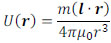
It is assumed that magnetic charges +m and -m are located at point P with a separation of l. The magnetic potential, U(r), as a function of the distance from the center of the above magnetic charges, r, is given by the following equation:
 |
(2) |
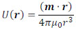
Here, μ0 (= 4π × 10-7 H/m) is the vacuum magnetic permeability. We deal with a vacuum environment instead of a human body for simplicity. In fact, we can use the value of μ0 for the human body permeability [21]. With the magnetic dipole moment m = ml, Eq. (2) is rewritten as
 |
(3) |
where (m · r) is the inner product of vectors m and r. Furthermore, it is assumed that |r| >> |l|. By differentiating U(r) with respect to r, we can obtain the magnetic field H(r) as
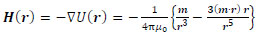 |
(4) |
Here, the point P(x, y, z) in Cartesian coordinates corresponds to P(r, ϕ, θ) in polar coordinates. Thus, the r, θ and ϕ components of H(r) are given by the following equations:
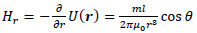 |
(5) |
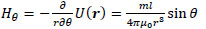 |
(6) |
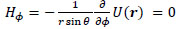 |
(7) |
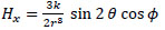
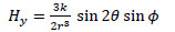
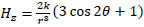
Taking the z-axis be in the direction of m, the x-, y- and z-axis components of H(r), Hx, Hy, and Hz, respectively, are given by the following equations:
 |
(8) |
 |
(9) |
 |
(10) |
With the new coefficient
 |
(11) |
Eqs. (8)-(10) are written as
 |
(12) |
 |
(13) |
 |
(14) |
Note that the sensitivity of magnetic field sensors should be well adjusted to obtain the position of the magnetic dipole with high accuracy. A magnetic sensor at an arbitrary position Q(X, Y, Z) can detect the magnetic field components not in the local coordinate system but in the global coordinate system. Thus, Eqs. (12)-(14) give the components in the local coordinate system. From Eq. (1),
 |
(15) |
Using Q(X, Y, Z), P(a, b, c), and m = (s, t, u) in global coordinates, Eq. (4) is rewritten as
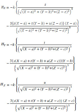 |
(16) |
Here, s, t, u are the unit X, Y, Z components for the orthogonal projection of m onto the global coordinate system, respectively, where
 |
(17) |
Equation (16) comprises the 5th degree nonlinear simultaneous equations with the constraint of Eq. (17). To obtain the solution of the simultaneous equations, methods such as the trust-region-step method [22],trust-region-dogleg method [23], and Levenberg-Marquardt method [24, 25] can be used. However, the calculation burden is rather large for these algorithms. To reduce the burden, a linear algorithm to calculate the position P(a, b, c) by 3-D magnetic field measurement was proposed in [10]. It was pointed out that at least five measurement points are required for accurate positioning.
Here we examine the magnetic field strength provided by a magnetic dipole. In this case, it is convenient to deal with this matter by considering the use of a solenoid coil [26]. It is well known that the magnetic flux, Φm, for an ideal solenoid with an infinite length is given by
 |
(18) |
where n is the number of turns, I is the current, S is the cross-sectional area of the solenoid coil, and d is its diameter. In this case, the induced electromotive force, V, is given by
 |
(19) |
Therefore, the self-inductance for a solenoid coil of infinite length, , is given by
 |
(20) |
Using Nagaoka’s coefficient, κ, the self-inductance of a finite-length solenoid coil, L, is given by [27].
 |
(21) |
where L∞ is the inductance of an infinite-length solenoid coil. κ is given by
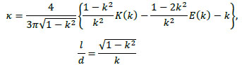 |
(22) |
where l and d are the length and diameter of the solenoid coil, respectively. Further, K(k) and E(k) are the complete elliptic integrals of the first kind and second kind, respectively, given by
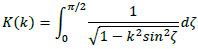 |
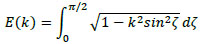 |
(23) |
Using the above solenoid, we can express the magnitude of the magnetic dipole moment as follows:
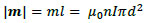 |
(24) |
where I is the electrical current in the solenoid coil. The magnetic flux density, B, and magnetic field, H, have the following relationship:
 |
(25) |
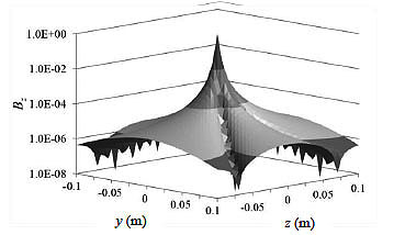
As mentioned later in this section, in the experiment, we use a solenoid coil with a diameter of 2.6 × 10⁻² m (thus, S ≈ 5.3 × 10⁻⁴ m2), a length of 4.0 × 10⁻² m, and n = 218. The measured resistance is 0.6 Ω. Thus, I = 0.83 A for a drive voltage of 0.5 V. With these parameters, the theoretical value of the magnetic flux density on the y-z plane is calculated using Eqs. (8)-(14) and (24). Fig. (3) shows the z-axis component of the magnetic flux density, Bz.
3.3. AI-Vased Positioning
AI includes fields such as Deep Learning (DL) and the Genetic Algorithm (GA) [28, 29]. DL is a class of machine learning (ML). In DL, sufficient learning is necessary for an efficient performance. For the adoption of this method for the positioning of a target within a human body, a propagation map of the human body is necessary. From the viewpoint of flexibility in prior learning, this method is not suitable. On the other hand, methods based on the GA do not require multiple learning to obtain satisfactory results.
Particle Swarm Optimization (PSO) is another candidate method for this purpose [30, 31]. In the case of a simple calculation for a moving target, the GA is suitable. Note that our objective is not to provide a comparison of the performances of the informed search methods such as PSO, Simulated Annealing (SA), and the GA but to show the potential of an AI- based method for practical positioning.
To reduce the difficulty of expressing the solution in binary code, the Real-Coded Genetic Algorithm (RCGA) [32] is used as the GA. In this method, after generating an initial population of possible real-valued solutions, to breed the next generation, some of the population is selected by considering the fitness of each gene. On the basis of the fitness, genetic manipulations such as crossover and mutation are performed. By carrying out iterative operations involving all genes, we can estimate the solution to a problem. Selection methods include roulette wheel selection, ranking selection, tournament selection, and elitism [33]. Crossover methods for the general GA include single-point crossover, n-point crossover, and uniform crossover [34, 35]. Mutation operators have also been reviewed [35].
In the RCGA, the gene type is expressed by real-number vectors instead of bit strings in the conventional GA. Mutation operators include uniform mutation and boundary mutation. With regard to the crossover, several methods have proposed such as blend crossover (BLX-α) [32], Unimodal Normal Distribution Crossover (UNDX) [36], Simplex Crossover (SPX) [37], and Parent Centric Recombination (PCX) [38]. Here, we use BLX-α. In this method, the child gene is determined from the parents’ genes in accordance with a uniform distribution. This method does not require a complex calculation, in contrast with other methods.
Using the above-mentioned RCGA, we propose a positioning method based on the magnetic field strength. A flowchart of the proposed method is shown in Fig. (4). For simplicity, we assume that multiple magnetic field sensors are placed around the outside of a human body. In Computer Tomography (CT), measurement points are located on the same plane to obtain a slice image of a human body. In our method, roulette wheel selection method is chosen with the value α = 0.2. The mutation rate is set as 0% for simplicity in our calculation. On the other hand, the crossover rate is set as 80%. The population size is set as 20.
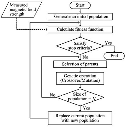
Fig. (5) shows the arrangement of magnetic field sensors. M magnetic field sensors are placed at equal-angle intervals. The x-axis is vertically in front of the paper surface. It is assumed that the target magnetic moment is at the origin of the local coordinate system, which corresponds to the point P(a, b) in the global coordinate system. The magnetic moment vector, m, given in Sec. 2 is on the z-axis. On the basis of the magnetic field strength at the measurement points, the position of the target is estimated using the GA with N genes. It is assumed that genes are randomly distributed within the circle.
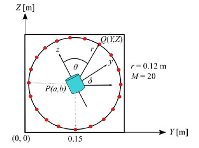
To simulate the transverse plane of a human body, we model a human body as a circular cylinder with a radius of r = 0.12 m. This value corresponds to the threshold value for the girth of the abdomen of 0.85 m, which is a diagnostic criterion for metabolic syndrome for men in Japan.
The initial population of possible solutions lies within the circle. The fitness function is given as
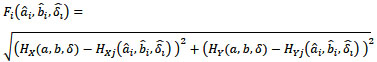 |
(26) |
Here, HX and HY are the X and Y components of the measured magnetic field strength in global coordinates, respectively. a and b are the true coordinate values of the target. ai and bi are coordinate values of the estimated position for the ith gene. δ and  are the true and estimated angles in global and local coordinates, respectively. Our method minimizes the value of the fitness function. With
  and δ = 0, the average position error, Ep, is given by
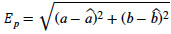 |
(27) |
In the same way, we define the average cosine angle error, Ea, as
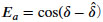 |
(28) |
Fig. (6) shows an example of the average position error vs the number of genes. A curve for random intervals is also illustrated for comparison. Here, the target is at the center of the circle. As the number of genes increases, the average position error decreases. The performance for equal intervals is slightly better than that for random intervals.
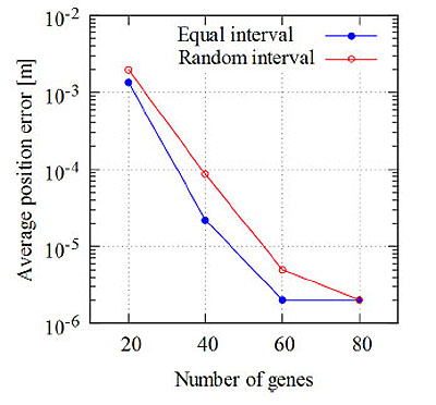
Fig. (7) shows an example of the average position error vs the number of measurement points. For both equal intervals and random intervals, as the number of measurement points decreases, the average position error increases. The average position error for equal intervals with M = 5 is about three times that with M = 20. The difference in the average position errors increases rapidly between δ = 0 and δ = π/4 for M = 3 in the case of equal intervals. On the other hand, in the case of random intervals, when M decreases from 20 to 3, the average position error increases by approximately two orders of magnitude.
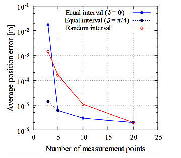
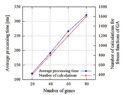
Fig. (8) shows an example of the average processing time for gene manipulation and the number of calculations vs the number of genes. In the RCGA method, the number of calculations is N×M. The average processing time is proportional to the number of genes. The processing time depends on the performance of the computer. In our computer simulation, a Windows 8.1/ 64-bit Personal Computer (PC) with an Intel® Pentium® G3250, 3.2 GHz CPU and 4 GB RAM was used. When the number of genes was 60, for example, the processing time was about 270 ms.
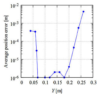
Figs. (9 and 10) respectively show the average position error when the target is moved vertically and horizontally from the center of the circle on the same plane. Fig. (9) shows the results for the case that the Y-axis is fixed as 0.15 m, and Fig. (10) shows the results for the case that the Z-axis is fixed as 0.15 m. Here, the measurement points are set at equal-angle intervals and the number of genes is N = 80.
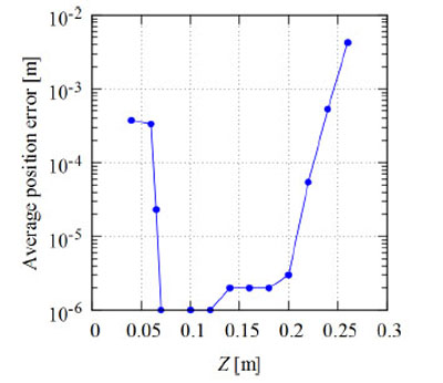
The average position error for a population size (number of genes) of N = 80 is given in Table 1 for different values of δ. As shown in this table, there are rather large positioning errors when δ = π/2 and 3π/2 of 20% and 17%, respectively. To reduce these errors, additional measurement with different points is desirable. As shown in Figs. (9 and 10), for the cases when the target is away from the center of the circle, the average position error increases. When Y = 0.15 m and Z = 0.27 m, for example, the average position error is about 0.004 m. When the Y-axis is between 0.03 and 0.23 m, the average position error is within 0.001 m. This value is 0.83% of the radius of the circle. These results show that we can obtain the position of the target with smaller errors by translation and rotation of the global coordinate axes. In this study, the computer simulation is conducted for two-dimensional space. We know that the average positioning error for 3-D space is the sum of the errors for each axis according to Eq. (27). Thus, we can conclude that the RCGA method is also effective in 3-D space.
| δ (rad) |  |
Average position error | Average cosine angle error |
|---|---|---|---|
| 0 | 7.43x10⁻³ | 2.00x10⁻⁶ | 0 |
| π /4 | 1.13x10-0 | 4.50x10⁻⁵ | 1.94x10⁻⁴ |
| π /2 | 1.67x10⁻¹ | 3.20x10⁻² | 1.20x10⁻⁵ |
| π | 2.25x10-0 | 3.50x10⁻⁵ | 4.08x10⁻⁴ |
| 3π /2 | 7.10x10⁻¹ | 2.65x10⁻² | 8.90x10⁻⁵ |
| 2 π | 1.92x10⁻² | 3.00x10⁻⁶ | 2.00x10⁻⁶ |
4. DISCUSSION
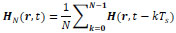
In medical engineering, to obtain the position of human brain activity, Electroencephalography (EEG) and MEG are used [39]. In these methods, the inverse position problem results in source estimation for Poisson equation [40, 41]. When we estimate the position of a moving target such as a capsule endoscope, the period of magnetic field strength measurement and the calculation speed should be taken into account. Within the processing time for estimation of Tp, the target moves away from the point of measurement by vTp (v: motion speed of the target). This effect causes an additional positioning error. The motion speed of a capsule endoscope, v, is 2 × 10⁻⁴ – 4 × 10⁻⁴ m/s. This value is calculated from the length of the small intestines [42] and the gastrointestinal transit time of 10 h [43]. Thus, the required estimation speed is given under the constraint of positioning error. If the maximum tolerance of the positioning error is 5 × 10⁻² m, for example, the total measurement time should be within 150 s. From a practical viewpoint, this value is sufficiently large to conduct measurement. Under practical measurement conditions, a capsule endoscope does not move in one direction at a constant speed. In this case, a moving-average approach is effective. For a sampling period of Ts and a measured magnetic field strength at time t, H(r, t), the moving average over N samples at time t, HN (r, t), is given by
 |
(29) |
where both H(r, t) and HN(r, t) are 3-D vectors, namely, H(r,t) = (Hx (x, t), Hy (y, t), Hz (z, t)) or H(r, t) = (Hr (r, t), Hθ (r, t), Hϕ (r, t)). In our method, the only information we can use the values of Hx, Hy, and Hz. To obtain accurate positioning results, we should take into consideration the sampling period and quantum noise in analogue-to-digital (A/D) conversion when collecting measurement data for computation. For a discussion of this matter, please refer to other books dealing with the digitization of analogue signals [44].
As mentioned before, multiple point measurement is effective for obtaining higher accuracy in the positioning. To accomplish multiple point measurement for a moving target, high-speed estimation with a low error is necessary. The adoption of the GA is effective for meeting this requirement. Furthermore, compressed sensing [45] can also be useful for solving the inverse problem in our proposed method. In this approach, we can obtain the position of the target based on the sparseness of the limited number of measurement data.
5. EXPERIMENTAL TEST MEASUREMENT
In this section, experimental test measurement results are provided to confirm the theoretical results. Without loss of generality, we assume a stationary target.
5.1. Measurement Test Setup
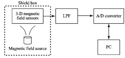
Fig. (11) is block diagram of the laboratory measurement test. The measurement was performed in an electromagnetically shielded room to avoid environmental interference [46]. The size of the room was W6.2 m × D5.2 m × H2.5 m, and the room attenuates transmission by more than 95 dB in the frequency range of 100 kHz - 10 GHz. MI-type magnetic field sensors were used to detect the magnetic field components [19]. According to the product catalogue, the nominal sensitivity of the sensors was 4 mV/μT. Instead of using a real capsule endoscope, we used a pseudo-capsule, in which some electronic circuits were installed.
This capsule was fixed at an arbitrary point using a ring stand inside a shield box with a size of 0.57 m × 0.38 m × 0.3 m. The shield box was made of cardboard which is covered with a magnetic shielding sheet (Hitachi Metals MS-F) [47]. There was a small amount of power consumed when the circuit was in operation. As a result, an additional magnetic field was superimposed on the background geomagnetic field. We estimated the position of the capsule using the collected 3-D magnetic field component data.
To obtain the characteristic of the magnetic sensor, we performed basic measurements for the stationary case. We prepared a solenoid coil driven by a sinusoidal signal with an amplitude of 0.5 V and a frequency of 1 kHz, to cancel the effect of the background magnetic field, as discussed in Sec. 2.1. To increase the magnetic field strength, we used a multiple-turn solenoid. The generated magnetic field strength at the center of both ends of the solenoid was estimated to be about 2.2 × 10⁻³ T. In the experiment, we used a solenoid with a diameter of 2.6 × 10⁻² m (thus S ≈ 5.3 × 10⁻⁴ m2), a length of 4.0 × 10⁻² m, and n = 218. The measured resistance was 0.6 Ω. The solenoid was fixed at the point P(0, 0) using a ring stand instead of fixing a magnetic field sensor. The sensor output signal was passed through a Low Pass Filter (LPF) to remove the signal with the frequency of 60 Hz induced by the Alternate Current (AC) line. We used buffer amplifiers because the sensors have lower output current capability. The amplified LPF output signal was fed into a PICO Technology® ADC16 A/D converter. The number of conversion bits was set as 16 bits by considering the range of the magnetic sensor output voltage. Digital data obtained every 100 ms were collected by a PC. Using these data, the position of the solenoid was calculated by newly developed application software written in C++ programming language.
5.2. Measurement Results
3-D positioning was carried out with a set of three magnetic field sensors at the measurement point in 3-D space.
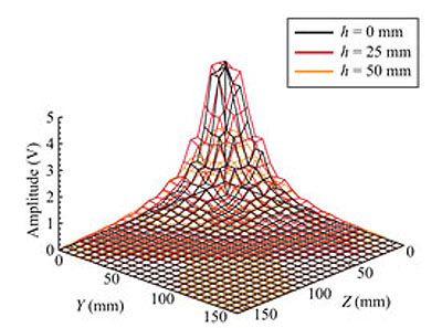
Fig. (12) shows an example of the measured z-axis component of the magnetic field, Hz, with h as a parameter, where h is the height of the measurement point from the y-z plane including the origin in Cartesian coordinates. The amplitude of 0 V corresponds to the background geomagnetic field. The direction of the maximum sensitivity of the sensor was forward the origin with a value of z = 0 mm. The amplitude of the sensor output, Voz, corresponds to Hz. As shown in this figure, the amplitude is increased when the sensor is moved to the origin along the z-axis. In the neighborhood of the origin, the measurement values for h = 25 mm are greater than those for h = 0 mm. This is because of the eccentricity of solenoid windings. For ideal circular windings, more regulated characteristics are expected. However, in a practical environment, the magnetic field distribution is not expected to be regulated as well as in our test measurement. Comparing this figure with Fig. (3), we find that the measured and theoretical magnetic field strengths are similar. Thus, using the measured values of the magnetic field strength, we can estimate the position of the target by using the previously mentioned GA method.
CONCLUSION
A positioning method for biosensor nodes such as capsule endoscopes was proposed. This method is based on magnetic field detection with the aid of the GA and provides the possibility of achieving accurate positioning with a low cost and simple procedure. A wireless communication method for effective signal exchange among sensor nodes is necessary for totally effective biosensor networks. The results of a study on this matter including in-vivo propagation will be proposed in the future.
LIST OF ABBREVIATIONS
| AI | = Artificial Intelligence |
| BAN | = Body Area Network |
| GA | = Genetic Algorithm |
| ICT | = Information and Communication Technology |
| IoT | = Internet of Things |
ETHICS APPROVAL AND CONSENT TO PARTICIPATE
Not applicable.
HUMAN AND ANIMAL RIGHTS
No animals / humans were used for the studies that are bases of this research.
CONSENT FOR PUBLICATION
Not applicable.
AVAILABILITY OF DATA AND MATERIALS
The authors confirm that the data supporting the findings of this research are available within the article.
FUNDING
This work was partly supported by Grant-in-Aid for Scientific Research (C)25420374 from Japan Society for the Promotion of Science (JSPS).
CONFLICT OF INTEREST
The authors declare that there is no conflict of interest, financial or otherwise.
ACKNOWLEDGEMENTS
The authors would like to thank Prof. Shuxiang Guo, Prof. Koji Ishii, and Prof. Hirotoshi Asano of Kagawa University for the fruitful collaboration.