All published articles of this journal are available on ScienceDirect.

A Comparative Study on the Influence of Probe Placement on Quality Assurance Measurements in B-mode Ultrasound by Means of Ultrasound Phantoms
Abstract
To check or to prevent failures in ultrasound medical systems, some tests should be scheduled for both clinical suitability and technical functionality evaluation: among them, image quality assurance tests performed by technicians through ultrasound phantoms are widespread today and their results depend on issues related to scanner settings as well as phantom features and operator experience. In the present study variations on some features of the B-mode image were measured when the ultrasound probe is handled by the technician in a routine image quality test: ultrasound phantom images from two array transducers are processed to evaluate measurement dispersion in distance accuracy, high contrast spatial resolution and penetration depth when probe is handled by the operator. All measurements are done by means of an in-house image analysis software that minimizes errors due to operator’s visual acuity and subjective judgment while influences of ultrasound transducer position on quality assurance test results are estimated as expanded uncertainties on parameters above (measurement reproducibility at 95 percent confidence level): depending on the probe model, they ranged from ±0.1 to ±1.9 mm in high contrast spatial resolution, from ±0.1 to ±5.5 percent in distance measurements error and from ±1 to ±10 mm in maximum depth of signal visualization. Although numerical results are limited to the two examined probes, they confirm some predictions based on general working principles of diagnostic ultrasound systems: (a) measurements strongly depend on settings as well on phantoms features, probes and parameters investigated; (b) relative uncertainty due to probe manipulation on spatial resolution can be very high, i.e. from 10 to more than 30 percent; (c) Field of View settings must be taken into account for measurement reproducibility as well as Dynamic Range compression and phantom attenuation.
1. INTRODUCTION
To check or to prevent failures in ultrasound medical systems, some tests should be scheduled for both clinical suitability and technical functionality evaluation: while clinical evaluation is mainly based on the subjective examination of specific test image sets, technical tests should be related to objective measurements of physical parameters. To this aim, ultrasound phantoms are useful to assess technical efficiency and performance changes in diagnostic ultrasound systems due to aging or damages that may occur in routine exams [1-10, 12-18]. In particular a tissue mimicking ultrasound phantom (US phantom) is a device that mimics human tissues properties in ultrasound wave propagation: its material has both sound velocity and attenuation similar to human tissues. US phantoms are often embedded with test objects, that are used to test both image quality and diagnostic device accuracy. By the way image quality assurance tests for medical ultrasound devices are usually based on measurements of specific parameters [1-7, 10, 15, 16] such as spatial resolution, low contrast penetration, accuracy in distance measurements and local dynamic range in imaging systems (B-mode, M-mode, 3D), as well as the estimation and display of blood velocity and sensitivity in echo Doppler systems [9, 12, 13]: routine tests are often performed by technicians using ultrasound phantoms and results depend on phantom features as well as scanner settings and operator manual skill and experience. In scientific literature the operator’s influence on tests precision seems not to be systematically evaluated and effects of the probe manipulation on ultrasound image parameters are not clear: in our work the influence of probe placement is evaluated for two different array transducers, when ultrasound probe is handled by the technician during the quality assurance test performed by using two different US phantoms.
2. MATERIALS AND METHODS
2.1. Ultrasound Signal Processing
To better understand the experimental results expressed in this work on quality assurance parameters, it is appropriate to touch on the echo processing from the ultrasound probe to the gray level on the monitor: every ultrasound image is produced by sending an ultrasound wave into a medium and collecting the reflected energy (i.e. ultrasound echoes); in 2D imaging (B-mode) reflected echoes amplitudes are converted into grayscale values of pixels in the ultrasound image. The main steps of the conversion above are outlined in Fig. (1).

Echo processing scheme. In the beam former, echoes from tissues are converted to electric signals by piezoelectric transducers PT, which are added in phase through delay lines DL and amplified by TGC. Echo signals are then demodulated, filtered and compressed in the signal processing section. In the image processing section, echoes are firstly converted into numeric values and arranged in the image matrix by the scan converter (pixels) and then pre-processed. After image has been saved, image pixel are postprocessed and displayed.
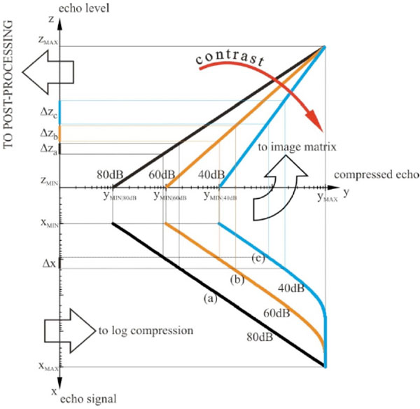
Dynamic compression of echoes. Echo signals from TGC are log compressed, saved into the image matrix and then postprocessed: (a) low compression curve (80dB Dynamic Range), (b) medium compression curve (60dB Dynamic Range), (c) high compression curve (40dB Dynamic Range).
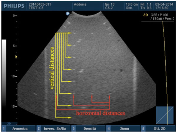
Accuracy in distance measurements. For each pair of point targets the measurement distance relative error between the nominal and the measured distance in the ultrasound image is calculated for both horizontal and vertical distances.
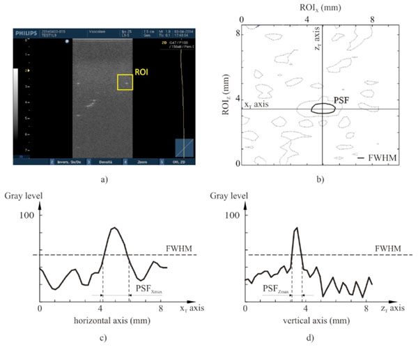
High contrast spatial resolution for each point target. The spatial resolution analysis is performed by an in-house software on gray levels within a ROI of the ultrasound image (a): a threshold algorithm at Full Width Half Maximum is applied to evaluate the PSF (b) and both its maximum width PSFXmax (c) and length PSFZmax (d).
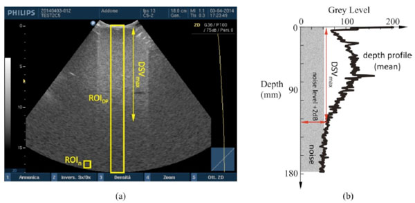
Maximum depth of signal visualization. (a) Two different ROIs in the ultrasound image are provided to evaluate DSVmax by software: the mean gray level in ROIn estimates the noise level, while DSVmax is determined as maximum distance from the probe surface where echo signal, displayed in ROIDP and plotted (b) on a depth profile of (mean) gray levels, is at +2dB over the noise level.
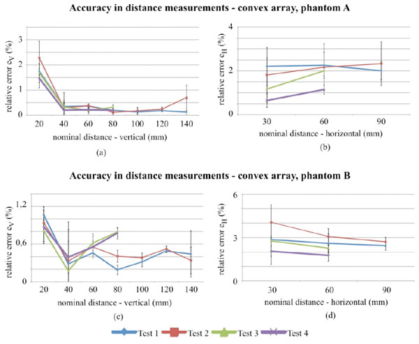
Accuracy in distance measurements for the convex array probe on phantom A and B, evaluated for different distances within the FoV. Differences in lengths of test 3 and test 4 curves are due to the smaller FoV.
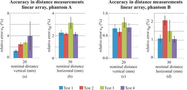
Accuracy in distance measurements for the linear array probe on phantom A and B, evaluated for a 20mm (vertical) and 30mm (horizontal) nominal distances.
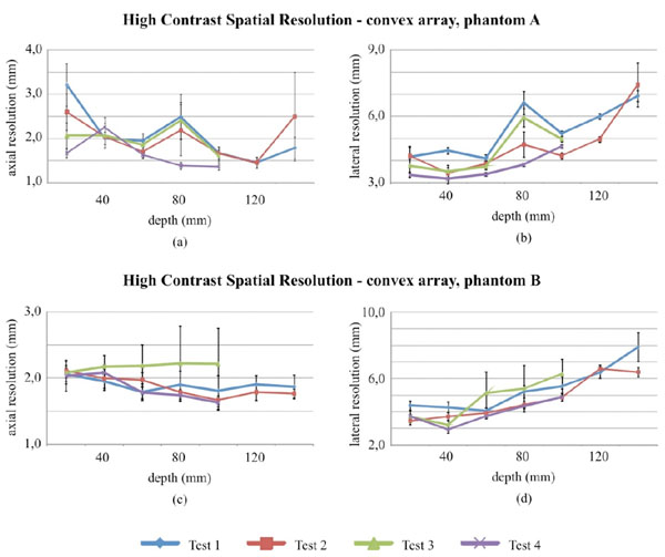
High contrast spatial resolution measurements for the convex array probe in Phantom A and B.

High contrast spatial resolution measurements for the linear array probe in phantom A and B.
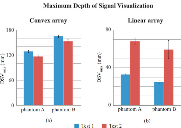
Maximum depth of signal visualization for convex array (a) and linear array probe (b).
Ultrasound phantoms characteristics.
| Model | GAMMEX 405 GSX LE (phantom A) |
GAMMEX 1425A (phantom B) |
|---|---|---|
| Dimensions and weight | ||
| Dimensions | 23.2×8.25×18.5 cm | 40.7 × 22.9 × 35.6 cm |
| Weight | Approx. 28 N | Approx. 100 N |
| Background Material | ||
| Speed of sound | 1540±10 m/s | 1540±10 m/s |
| Attenuation | 0.7±0.05 dB/cm/MHz | 0.5±0.05 dB/cm/MHz |
| Pin targets | ||
| Diameter | 0.1 mm | 0.1 mm |
| Vertical spacing | 2 cm at 2–16 cm deep | 2 cm at 3–17 cm deep |
| Horizontal spacing | 3 cm at 2–12 cm deep | 3 cm at 3–13 cm deep |
Measurements settings for probe 1 (convex array).
| PROBE 1 (convex array) | ||||
|---|---|---|---|---|
| Test 1 a | Test 2 a | Test 3 b | Test 4 b | |
| Nominal Frequency range (MHz) | 2-5 | |||
| Field of View (mm) | 180 | 180 | 110 | 110 |
| Dynamic Range (dB) | Maximum | Medium | Maximum | Medium |
| Focus depth (mm) | 70 | |||
| Overall gain | Medium | |||
| Transmit Power | Maximum | |||
| Pre-processing: edge enhancement | Minimum | |||
| Pre-processing: persistence | Minimum | |||
| Pre-processing: zoom | No | |||
| Post-processing | Linear | |||
| Phantom | A, B | |||
Measurements settings for probe 2 (linear array).
| PROBE 2 (linear array) | ||||
|---|---|---|---|---|
| Test 1 a | Test 2 a | Test 3 b | Test 4 b | |
| Nominal Frequency range (MHz) | 5-9 | |||
| Field of View (mm) | 75 | 75 | 50 | 50 |
| Dynamic Range (dB) | Maximum | Medium | Maximum | Medium |
| Focus depth (mm) | 20 | |||
| Overall gain | Medium | |||
| Transmit Power | Maximum | |||
| Pre-processing: edge enhancement | Minimum | |||
| Pre-processing: persistence | Minimum | |||
| Pre-processing: zoom | No | |||
| Phantom | A, B | |||
a Maximum Depth of Penetration, Accuracy in distance measurements (vertical and horizontal), High contrast spatial resolution (lateral and axial)
b Accuracy in distance measurements (vertical and horizontal), High contrast spatial resolution (lateral and axial).
Accuracy in distance measurements for the convex array probe (min-max range over the 4 tests). For every distance and test considered, accuracy is calculated by averaging relative error values over the images of the same group.
| Convex array | ||
|---|---|---|
| x-axis (horizontal) | z-axis (vertical) | |
| Accuracy in distance measurements (%) | 0.6 ÷ 2.3 (Ph.A) 1.8 ÷ 4.0 (Ph.B) |
0.1 ÷ 2.3 (Ph.A) 0.2 ÷ 1.1 (Ph.B) |
Uncertainty on accuracy in distance measurements for the convex array probe (min-max range over the 4 tests). For every distance and test considered, accuracy is calculated by averaging relative error values over the images of the same group.
| Convex array | ||
|---|---|---|
| x-axis (horizontal) | z-axis (vertical) | |
| Accuracy in distance measurements (%) | ±0.3 ÷ ±1.1 (Ph.A) ±0.4 ÷ ±1.2 (Ph.B) |
±0.4 ÷ ±0.7 (Ph.A) ±0.2 ÷ ±0.6 (Ph.B) |
Influence of settings on accuracy in vertical distance measurements for the convex array probe: p-values for Kruskal- Wallis test
| CONVEX ARRAY | Accuracy in vertical distance measurements, phantom A | ||||||
|---|---|---|---|---|---|---|---|
| distance (mm) | 20 | 40 | 60 | 80 | 100 | 120 | 140 |
| Test 1 | Not Significant | Not Significant | p=0.002 (1) |
p=0.01 (2) |
Not Significant | Not Significant | p=0.001 (3) |
| Test 2 | |||||||
| Test 3 | - | - | - | ||||
| Test 4 | |||||||
| CONVEX ARRAY | Accuracy in vertical distance measurements, phantom B | ||||||
| distance (mm) | 20 | 40 | 60 | 80 | 100 | 120 | 140 |
| Test 1 | p=0.02 (4) |
Not Significant | Not Significant | p<0.0001 (5) |
p=0.04 (6) |
Not Significant | Not Significant |
| Test 2 | |||||||
| Test 3 | - | - | - | ||||
| Test 4 | |||||||
(1) Significant difference between Test 3 and both Test 1 and Test 2. Significant difference between Test 2 and Test 4; (2) Significant difference between Test 2 and Test 3; (3) Significant difference between Test 1 and Test 2; (4) Significant difference between Test 1 and Test 4; (5) Significant difference between Test 3 and Test 4. Significant difference between Test 2 and both Test 3 and Test 4; (6) Significant difference between Test 1 and Test 2
Influence of settings on accuracy in horizontal distance measurements for the convex array probe: p-values for Kruskal- Wallis test.
| CONVEX ARRAY | Accuracy in horizontal distance measurements, phantom A | ||
|---|---|---|---|
| distance (mm) | 20 | 40 | 60 |
| Test 1 | p=0.003 (1) |
p=0.003 (2) |
Not Significant |
| Test 2 | |||
| Test 3 | - | ||
| Test 4 | |||
| CONVEX ARRAY | Accuracy in horizontal distance measurements, phantom B | ||
| distance (mm) | 20 | 40 | 60 |
| Test 1 | Not Significant | Not Significant | Not Significant |
| Test 2 | |||
| Test 3 | - | ||
| Test 4 | |||
(1) Significant difference between Test 4 and both Test 1 and Test 2.
(2) Significant difference between Test 4 and both Test 1 and Test 3.
Accuracy in distance measurements for the linear array probe (min-max range over the 4 tests).
| Linear array | ||
|---|---|---|
| x-axis (horizontal) | z-axis (vertical) | |
| Accuracy in distance measurements (%) | 2.1 ÷ 3.1 (Ph.A) 1.1 ÷ 2.1 (Ph.B) |
0.8 ÷ 7.4 (Ph.A) 0.3 ÷ 8.7 (Ph.B) |
Uncertainty on accuracy in distance measurements for the linear array probe (min-max range over the 4 tests).
| Linear array | ||
|---|---|---|
| x-axis (horizontal) | z-axis (vertical) | |
| Accuracy in distance measurements (%) | ±0.1 ÷ ±0.5 (Ph.A) ±0.1 ÷ ±0.6 (Ph.B) |
±0.2 ÷ ±5.5 (Ph.A) ±0.1 ÷ ±3.0 (Ph.B) |
Influence of settings on accuracy in vertical and horizontal distance measurements for the linear array probe: p-values for Kruskal-Wallis test.
| LINEAR ARRAY | Phantom A | |
|---|---|---|
| Accuracy in vertical distance measurements | Accuracy in horizontal distance measurements, | |
| distance (mm) | 20 | 30 |
| Test 1 | p<0.0001 (1) |
p=0.0007 (3) |
| Test 2 | ||
| Test 3 | ||
| Test 4 | ||
| Phantom B | ||
| Test 1 | p=0.001 (2) |
p<0.0001 (4) |
| Test 2 | ||
| Test 3 | ||
| Test 4 | ||
(1) Significant difference between Test 1 and all the others;
(2) Significant difference between Test 1 and Test 2;
(3) Significant difference between Test 3 and all the others;
(4) Significant difference between Test 1 and all the others.
High contrast spatial resolution measurements for the convex array probe (min-max range over the 4 tests).
| Convex array | ||
|---|---|---|
| x-axis (lateral res.) | z-axis (axial res.) | |
| High Contrast Spatial resolution (mm) | 3.2 ÷ 7.4 (Ph.A) 3.9 ÷ 7.9 (Ph.B) |
1.4 ÷ 3.2 (Ph.A) 1.6 ÷ 2.2 (Ph.B) |
Uncertainty on high contrast spatial resolution measurements for the convex array probe (min-max range over the 4 tests).
| Convex array | ||
|---|---|---|
| x-axis (lateral res.) | z-axis (axial res.) | |
| High Contrast Spatial resolution (mm) | ±0.3 ÷ ±1.9 (Ph.A) ±0.3 ÷ ±1.4 (Ph.B) |
±0.2 ÷ ±1.0 (Ph.A) ±0.2 ÷ ±0.6 (Ph.B) |
Influence of settings on axial resolution for the convex array probe: p-values for Kruskal-Wallis test.
| CONVEX ARRAY | High contrast axial resolution, phantom A | ||||||
|---|---|---|---|---|---|---|---|
| depth (mm) | 20 | 40 | 60 | 80 | 100 | 120 | 140 |
| Test 1 | p<0.0001 (1) |
Not Significant | p=0.003 (2) |
p<0.0001 (3) |
p=0.0004 (4) |
Not Significant | Not Significant |
| Test 2 | |||||||
| Test 3 | - | - | |||||
| Test 4 | |||||||
| CONVEX ARRAY | High contrast axial resolution, phantom B | ||||||
| depth (mm) | 20 | 40 | 60 | 80 | 100 | 120 | 140 |
| Test 1 | Not Significant | Not Significant | p=0.004 (5) |
p=0.004 (6) |
Not Significant | Not Significant | Not Significant |
| Test 2 | |||||||
| Test 3 | - | - | |||||
| Test 4 | |||||||
(1) Significant difference between Test 1 and both Test 3 and Test 4. Significant difference between Test 2 and Test 4; (2) Significant difference between Test 1 and Test 4; (3) Significant difference between Test 4 and all the others; (4) Significant difference between Test 4 and all the others; (5) Significant difference between Test 4 and Test 3; (6) Significant difference between Test 4 and Test 3
Influence of settings on lateral resolution for the convex array probe: p-values for Kruskal-Wallis test.
| CONVEX ARRAY | High contrast lateral resolution, phantom A | ||||||
|---|---|---|---|---|---|---|---|
| depth (mm) | 20 | 40 | 60 | 80 | 100 | 120 | 140 |
| Test 1 | P=0.002 (1) |
p<0.0001 (2) |
p<0.0001 (3) |
p<0.0001 (4) |
p<0.0001 (5) |
p<0.0001 (6) |
Not Significant |
| Test 2 | |||||||
| Test 3 | |||||||
| Test 4 | |||||||
| CONVEX ARRAY | High contrast lateral resolution, phantom B | ||||||
| depth (mm) | 20 | 40 | 60 | 80 | 100 | 120 | 140 |
| Test 1 | Not Significant | Not Significant | p=0.004 (5) |
p=0.004 (6) |
Not Significant | Not Significant | Not Significant |
| Test 2 | |||||||
| Test 3 | |||||||
| Test 4 | |||||||
(1) Significant difference between Test 4 and both Test 1 and Test 2; (2) Significant difference between Test 1 and all the others; (3) Significant difference between Test 4 and both Test 1 and Test 2; (4) Significant difference between Test 4 and both Test 1 and Test 3; (5) Significant difference between Test 1 and both Test 2 and Test 4. Significant difference between Test 2 and all the others; (6) Significant difference between Test 1 and Test 2.
High contrast spatial resolution measurements for the linear array probe (min-max range over the 4 tests).
| Linear array | ||
|---|---|---|
| x-axis (lateral res.) | z-axis (axial res.) | |
| High Contrast Spatial resolution (mm) | 0.9 ÷ 2.5 (Ph.A) 1.3 ÷ 4.2 (Ph.B) |
0.7 ÷ 1.3 (Ph.A) 0.6 ÷ 1.6 (Ph.B) |
Uncertainty on high contrast spatial resolution measurements for the linear array probe (min-max range over the 4 tests).
| Linear array | ||
|---|---|---|
| x-axis (lateral res.) | z-axis (axial res.) | |
| High Contrast Spatial resolution (mm) | ±0.1 ÷ ±0.3 (Ph.A) ±0.3 ÷ ±1.4 (Ph.B) |
±0.1 ÷ ±0.2 (Ph.A) ±0.1 ÷ ±0.4 (Ph.B) |
Influence of settings on axial and lateral resolution for the linear array probe: p-values for Kruskal-Wallis test.
| LINEAR ARRAY | Phantom A | |
|---|---|---|
| High contrast axial resolution | High contrast lateral resolution | |
| depth (mm) | 40 | 40 |
| Test 1 | p=0.005 (1) |
p=0.001 (3) |
| Test 2 | ||
| Test 3 | ||
| Test 4 | ||
| Phantom B | ||
| Test 1 | p=0.004 (2) |
p<0.04 (4) |
| Test 2 | ||
| Test 3 | ||
| Test 4 | ||
(1) Significant difference between Test 1 and all the others; (2) Significant difference between Test 3 and Test 1;
(2) Significant difference between Test 3 and Test 1; (4) Significant difference between Test 3 and Test 2.
DSVmax for convex and linear array probe (min-max range over the 4 tests).
| Convex array | Linear array | |
|---|---|---|
| Maximum depth of signal visualization DSVmax (mm) | 117 ÷ 129 (Ph.A) 153 ÷ 165 (Ph.B) |
33 ÷ 69 (Ph.A) 25 ÷ 59 (Ph.B) |
Uncertainty on DSVmax for convex and linear array probe (min-max range over the 4 tests).
| Convex array | Linear array | |
|---|---|---|
| Maximum depth of signal visualization DSVmax (mm) | ±2 ÷ ±4 (Ph.A) ±1 ÷ ±4 (Ph.B) |
±1 ÷ ±4 (Ph.A) ±1 ÷ ±10 (Ph.B) |
Influence of settings on maximum depth of signal visualization for the convex array probe: p-values for Kruskal-Wallis test.
| Maximum Depth of Signal Visualization | ||
|---|---|---|
| CONVEX ARRAY | LINEAR ARRAY | |
| FoV (mm) | 180 | 75 |
| Phantom A | ||
| Test 1 | p<0.0001 (1) |
p<0.0001 (1) |
| Test 2 | ||
| Phantom B | ||
| Test 1 | p<0.0001 (1) |
p<0.0001 (1) |
| Test 2 | ||
(1) Significant difference between Test 1 and Test 2
Maximum uncertainty ranges for both of the probes.
| Convex array | Linear array | |
|---|---|---|
| Accuracy in distance measurements (%) | Hor. ±0.4 ÷ ±1.2 (Ph.B) Vert. ±0.4 ÷ ±0.7 (Ph.A) |
Hor. ±0.1 ÷ ±0.6 (Ph.B) Vert. ±0.2 ÷ ±5.5 (Ph.A) |
| High Contrast Spatial resolution (mm) | Axial res. ±0.2 ÷ ±1.0 (Ph.A) Lat. Res. ±0.3 ÷ ±1.9 (Ph.A) |
Axial res. ±0.1 ÷ ±0.4 (Ph.B) Lat. Res. ±0.3 ÷ ±1.4 (Ph.B) |
| Maximum depth of signal visualization DSVmax (mm) | ±1 ÷ ±4 (Ph.B) | ±1 ÷ ±10 (Ph.B) |
For each ultrasound pulse transmitted into tissues, the array probe receives a sequence of echoes that contains information related to the variation of the acoustical properties of the tissue. The time delays depend on the distance from the echo source to the probe emitting surface. Ultrasound echoes are converted into electric signals by piezoelectric transducers PT within the array probe.
In Fig. (1), the scanning is performed by the beam former, which sets the time delay for each piezoelectric transducer PT within the array probe and sums echo signals in phase to build a RF line of sight1. The electric signal above (e.g. about 90dB Dynamic Range) is firstly logarithmically amplified by means of the Time Gain Compensation (TGC) to compensate the attenuation of the investigated medium (e.g. about 50dB), then it is filtered and demodulated in order to increase the SNR (signal processing section in Fig. 1). In spite of the TGC action, amplified echo amplitudes change over a wide range (e.g. approximately a 100:1 ratio between the strongest and the weakest echo [2]) . To display them a compression is needed (to match the lower dynamic range of the display device, e.g. 20dB).
A scheme of the dynamic compression of echoes is shown in Fig. (2): a same difference Δx in echo signal from TGC can be log-compressed using three different compression curves (a), (b) and (c) to three different echo level intervals Δza, Δzb and Δzc in the image matrix. The stronger is the compression of Δx, the wider is the echo range Δz (i.e. gray level) in the image with a higher average value, therefore, echoes are displayed with higher contrast and brightness. This is important because by compression the low amplitude echoes can be enhanced in the image, as well as image noise. Then compressed echoes are arranged in the image matrix by means of the scan converter, and before storing it some processing is applied in order to improve image quality and details (pre-processing 2).
After image storage, collected data are interpolated and converted into brightness by means of a post-processing curve and digital-to-analog conversion (D/A): the ultrasound digital image is finally displayed on the monitor of the scanner. Images used in the present work are stored in a lossless format to avoid nonlinearities due to format compression.
2.2. Ultrasound Phantom
In the present work two Point Spread Function (PSF) Phantoms models are used for image quality assessment of a real time B-mode scanner, GAMMEX 405 GSX LE (phantom A) and GAMMEX 1425A (Phantom B). Both of them made by a tissue mimicking material embedded with nylon wires (whose transversal sections are considered as point target in the ultrasound image), low scatter targets (cystic masses) and gray scale targets (only phantom A), whose characteristics are shown in Table 1.
From Table 1, it can be observed that both phantoms have the same speed of sound and very similar pin targets arrangement (along both vertical and horizontal directions with the same spacing) but very different attenuation (phantom A attenuation is almost 40 percent higher than phantom B) and dimensions (phantom B is bigger and heavier than phantom A, with a wider transversal section).
2.3. Measurement Set-up
The measurement setup includes an ultrasound scanner Philips HD3, an array probe on the ultrasound phantom and a notebook pc for data acquisition and processing. Tests are performed with two different models of array probe (convex and linear array) on two tissues mimicking phantoms3 (see Table 1 for specifications) by a single operator. In particular, our study focuses on evaluation of the follow image quality parameters: (a) accuracy in distance measurements (both vertical and horizontal directions) [3, 5], (b) high contrast spatial resolution (both lateral and axial resolution) [5] and (c) maximum depth of signal visualization (or maximum depth of penetration) [6-8, 18]. The ultrasound probe is applied on the phantom by hand and its position is manually adjusted to clearly display test objects in the US image (no holder is used), then a single image is acquired and exported on a peripheral in a TIFF or DICOM format (lossless): for each phantom the whole procedure is repeated from 11 to 16 times. Therefore for a same test (Tables 2 and 3) a group of 11 up to 16 ultrasound images is provided and processed by an in-house software package, developed in a Matlab environment [3, 5-10, 15] to evaluate the variation of the parameters (a), (b) and (c) due to the probe manipulation on the phantom surface and whose operating principles are explained in the following paragraphs. The use of self-produced software is mainly due to economic reasons and transparent management of data processing, although comparable products are available on the market [17]. Settings are chosen to display the maximum number of test objects at the central frequency of the ultrasound probe (working frequency). Moreover all images are acquired within ±2° tilt angle, at medium overall gain and linear post processing while persistence, edge enhancement and other image processing are set to minimum.
To understand the settings better in Table 2 some definitions are reported below [5-9]:
• Nominal Frequency (of a transducer): acoustic working frequency of a transducer as quoted by the designer or manufacturer. In our study the ultrasound scanner provides a nominal frequency range, i.e. 2-5 MHz and 5-9MHz for the convex and linear array probe respectively.
• Field of View (FoV): area in the ultrasonic scan plane from which ultrasound information is acquired to produce one image frame. Since for each probe the diagnostic image size (in pixel) is quite constant, a FoV variation is associated to a different scale factor (mm to pixel ratio) and could influence other image characteristics, i.e. spatial resolution, accuracy in distance measurements.
• Focus Depth: nominal depth of the transmission focus in the ultrasound image. Each transmission focus is usually marked on the diagnostic image.
• Dynamic range (global): ratio of the maximum to the minimum echo-signal amplitude, even with changes of settings, that a scanner can process without distortion of the output signal.
• Local Dynamic Range: ratio, expressed in decibels, of the minimum echo amplitude that yields the maximum gray level in the digitized image to that of the echo that yields the lowest gray level at the same location in the image and the same settings. Local Dynamic Range influences image contrast and can be controlled by the operator (i.e. through dynamic range or compression settings).
• Gray Scale Mapping Function (GSMF): relationship between echo amplitudes and gray levels on the image. From GSMF the Local Dynamic Range can be estimated.
• Overall gain: the overall gain control amplifies all echo signals equally, irrespective of when they return to the transducer. Increasing the overall gain cannot improve significantly the Signal to Noise Ratio (SNR), because noise and signal are both amplified.
• Transmit Power: the transmit power controls the amplitude of pulses transmitted by the transducer. As the transmit power increases, echoes amplitudes grow, usually with a better Signal to Noise Ratio (SNR). On the other hand, by reducing the transmit power the exposure of the patient to ultrasound decreases and so the risk of any adverse effect (ALARA principle).
• Pre-processing - edge enhancement: a spatial high-pass filter to enhance the appearance of anatomical features in the ultrasound image.
• Pre-processing – persistence: it is a frame averaging to suppress random image noise.
• Pre-processing – zoom (read zoom): it is a way of magnifying a part of the ultrasound image, to overcame the inefficient use of the screen area when the imaged depth is larger than the imaged width and anatomical features appear small on the display.
• Post-processing: mapping functions that relate echo amplitudes to displayed brightness levels.
2.4. Accuracy in Distance Measurements
Vertical and horizontal distances are measured “from peak to peak” of the wires sections within the two phantoms and compared with their nominal values by an in-house software [3]: in particular, after the ultrasound image is processed in a workstation, first, the scale factor is automatically calculated from FoV then the operator is asked to choose n test object pairs by clicking on the image without care about centering each target because their barycentric coordinates are automatically calculated within a Region of Interest (ROI). These latter are then used for measuring the distance between each pair of wires, so errors due to operator subjectivity can be neglected. Therefore, the measurement distance relative error ek=|srk−smk|/srk×100 between the nominal (srk) and the measured distance (smk) in the image is calculated for each pair (k=1, 2, ...n) along both horizontal and vertical distances [3, 11]. For the k-th distance and for each test, the accuracy in distance measurements is calculated by averaging relative error values ek over the images of the same group Fig. (3).
Since distance accuracy depends on the difference between the effective acoustic velocities of the medium and the acoustic velocity used to calibrate the scanner, as well as on image scan conversion, scanning geometry and pixel dimensions [3], a dependence on FoV settings is expected with different results between horizontal and vertical distances.
2.5. High Contrast Spatial Resolution
High-contrast resolution characteristics can be evaluated locally from the size of the point-spread function (PSF), that is the characteristic response of the imaging system to a high-contrast point target: PSFs can be displayed by imaging high reflection targets that are smaller than one wavelength, as the nylon wires sections in the US phantoms that have been used in this work. In diagnostic ultrasounds the PSF is not isotropic, with different lateral and axial dimensions in the FoV, depending on distance from the transducer emitting surface: in other words, spatial resolution features change with position and depth in the US image, therefore many measurements of the lateral and axial diameters of the displayed wires sections are performed at different positions and depths (by the in-house software for all the settings in Table 2) to achieve the ultrasound system’s lateral and axial resolutions. In particular every wire section k (point target) in the US image is processed by a threshold algorithm at Full Width Half Maximum to evaluate both its maximum length PSFZmax(k) and width PSFXmax(k), whose values are assigned as high contrast axial and lateral resolution respectively Fig. (4).
Since PSF measurement depends also on pixel dimension and contrast between point target and tissue background, a dependence on FoV settings and phantom attenuation is expected with different results between horizontal and vertical dimensions.
2.6. Maximum Depth of Penetration
Maximum depth of penetration or Maximum Depth of Signal Visualization (DSVmax) is the maximum depth at which echo signals from scattering within a tissue-mimicking phantom can be detected [6-8, 15, 18]. In particular, DSVmax is achieved from a depth profile of gray levels within a ROIDP of 30 pixel width4 in the US image, by means of a threshold at 2dB [8] above the mean value displayed in a 10×10 pixel ROIn positioned at the end of the FoV5 (Fig. 5). To evaluate the +2dB threshold, the relationship between gray levels and echo amplitudes (dB) in the image is needed [8]: to this aim a GSMF is provided by means of the method proposed in [10] for each probe and dynamic range setting in Table 2. The method above is implemented in a specific software tool developed by the authors [15] to provide measurement results of DSVmax.
Since DSVmax measurement depends on SNR ratio (between speckle signal and electronic noise), a dependence on dynamic range settings and phantom attenuation is expected.
3. RESULTS AND DISCUSSION
For each of the above-mentioned parameters results are organized by probe and phantom model. Since all measurements are conducted through an image analysis software that minimizes errors due to operator’s subjective judgment and visual acuity, principal causes of results dispersion can be related to small image variations due to manual probe placement on the phantom surface. Therefore in our study influences of ultrasound transducer manipulation on quality assurance measurements are estimated through expanded uncertainties, evaluated as measurement reproducibility [11] at 95 percent confidence level (Students-t distribution).
Moreover a hypothesis test is carried out to verify whether the differences in the measurements of the three image parameters are statistically significant or not: since data do not meet assumptions of parametric statistics, the Kruskal-Wallis non parametric method is used with a post hoc analysis based on Dunnet’s test; results are reported in terms of p-values6 [19].
3.1. Accuracy in Distance Measurements
Accuracy in distance measurements is evaluated for the settings in Table 2 and 3 as expressed in section 2.4: measurements ranges and their uncertainty are shown in Tables 4 and 5, diagrams are plotted in Fig. (6).
In Fig. (6) results for the convex probe are shown: for vertical measurements no significant differences between tests are observed, while for horizontal distances (Fig. 6b and Fig. 6d) discrepancies between phantoms can be noticed. Moreover a slight difference in the horizontal distance relative error between tests (i.e. test 2, test 4) seems to confirm a FoV influence on results at lower dynamic ranges. To evaluate the test influences on measurement reproducibility a Fisher test (p-value<0.05) has been performed for results at horizontal-60mm and vertical-80mm distance: although in vertical distance measurements no significant differences can be observed among variances, in horizontal ones homoscedasticity should be rejected for both of phantoms, therefore a variation in measurement reproducibility related to test settings can be supposed. Measurements uncertainty ranges from ±0.3 to ±1.2 percent for horizontal distances, ±0.2 to ±0.7 percent for vertical distances. A hypothesis test has been done to verify whether the differences in accuracy measurements are statistically significant: results of the Kruskal-Wallis non parametric method and the Dunnet’s test post hoc analysis are reported in Tables 6 and 7 and a significant difference among test is found for both phantoms depending on distances.
Results for the linear array probe are shown in Fig. (7) and no significant differences are noticed for most of the measurements (see also Tables 8 and 9), nevertheless the F-test (p-value<0.05) indicates no equality of variances on horizontal (30mm, both of the phantoms) and vertical distances (20 mm, phantom A). Measurements uncertainty ranges from: ±0.1 to ±0.6 percent for horizontal distances, ±0.1 to ±5.5 percent for vertical distances. As seen for the convex array probe, a hypothesis test is performed on accuracy measurements for the linear array and results are shown in Table 10.
For the convex array transducer the differences between tests in horizontal distance can be attributed to phantom tissue mimicking material and mostly to FoV settings (Fig. 6b and Fig. 6d), because it influences mm to pixel ratio (i.e. scale factor) and the distortion of imaged nylon wires sections. In fact at lower FoVs, wires are selected near to the image boundaries, where distortion artifacts are stronger and become more evident for higher contrasts (i.e. Dynamic Range settings). All the above causes are likely to affect the measurement reproducibility, because of the enhancement of slight differences in the acquired images and their processing by the analysis software. Analogous considerations can be done for the linear array transducer, where high noise levels add dispersion to results. In particular, a singular dispersion is observed for vertical distance error ev in test 4 of Fig. (7a), likely due to a combined effect of the higher attenuation in phantom A and the increased noise with Dynamic Range reduction, that involved a reduced pin target visibility and software failures in barycentric calculus.
3.2. High Contrast Spatial Resolution
Lateral and axial resolution at FWHM are evaluated for settings in Table 2 and 3. Convex array measurements results are plotted in Fig. (8) and summarized in Tables 11 and 12.
In particular no significant variations between tests have been noticed for most of lateral and axial measurements of the convex array probe (Fig. 8), nevertheless some discrepancies between test can be observed in phantom A. A Fisher test (p-value<0.05) has been performed on parameter variances at 100 mm (both for lateral and axial resolution) and suggests that for results in Fig. (8c and Fig. 8d) (phantom B) homoscedasticity should be excluded. Measurements uncertainty ranges from: ±0.3 mm to ±1.9 mm for lateral resolution, ±0.2 mm to ±1.0 mm for axial resolution. Results of the hypothesis tests on spatial measurements are shown for both probes in Tables 13, 14 and 17.
Linear array spatial measurements are shown in Fig. (9) and no significant discrepancies can be noticed for most of the measurements, nevertheless no equality of variances, on both axial and lateral resolution values with the phantom B, are suggested by the F-test. Measurements results and uncertainty ranges are shown in Tables 15 and 16: uncertainties range from ±0.1 mm to ±1.4 mm for lateral resolution, from ±0.1 mm to ±0.4 mm for axial resolution. Differences between tests can be likely due to electrical noise level (whose display depends on Dynamic Range settings), phantom tissue mimicking material (attenuation) and FoV variation, because of its influence on both the scale factor and the pixelation error. As in distance evaluations, measurement reproducibility likely depends on all the above causes, because of the enhancement of differences among tested images.
3.3. Maximum Depth of Penetration
DSVmax is evaluated for settings 1 and 2 in Table 2 and 3: results are plotted in Fig. (10) and reported in Tables 18 and 19.
In Fig. (10a) a significant disagreement between phantoms is noticed for both the settings in the convex array probe: higher penetration depths are related to phantom B and measurements uncertainty ranges from ±1 mm to ±4 mm. On the other hand the F-test (p-value<0.05) suggests that homoscedasticity should be refused for phantom B tests. In Fig. (10b) a considerable discrepancy in results between tests and phantom has been observed for the linear array probe: higher penetration depths are consistent to each other and related to settings 2 for both of the phantoms and measurements uncertainty ranges from ±1 mm to ±10 mm, while variances should be considered non-homogeneous between tests for both of phantoms. In the convex array DSVmax seems to depend mostly on phantom model than test settings, on the other hand it is more settings dependent in linear array examinations while differences between phantom tests are not significant. As in the previous sections, a hypothesis test (Kruskal-Wallis) has been carried out to verify whether differences in maximum depth of penetration measurements are statistically significant: p-values are reported in Table 20 and showed significant differences between tests for both the phantoms.
4. DISCUSSION
Even if measurement uncertainties strongly depend on probe and phantom models, as well as parameter investigated and scanner settings, some general considerations can be drawn. In particular, for both convex and linear arrays the differences among test results seem to depend significantly on phantom tissue mimicking material, Dynamic Range and Field of View settings.
In fact, phantom A attenuation is more than 40 percent greater than that of phantom B so pin target imaging could be less visible and smoother over the background speckle, that is often related to a lower reproducibility and a higher uncertainty in parameter measurement (e.g. accuracy in distance measurements, spatial resolution). Moreover distortion artifacts are more intense and become more noticeable for higher contrasts, so they are dependent on dynamic range compression as well as noise: in some cases (i.e. linear array) noise increasing with dynamic range reduction is dramatic and influences image features measurements as Spatial Resolution and DSVmax significantly (see. Fig. 9c, Fig. 10b). Although FoV settings are related to the scale factor (mm to pixel ratio), which is is a meaningful parameter in image quality assessment. The measurements values and uncertainties seem to depend considerably on superposition of attenuation effects and dynamic range settings.
Maximum uncertainties ranges are summarized in Table 21, where vertical distance measurements for both the probes are likely influenced by effects on target visibility due to the higher attenuation in phantom A. On the other hand, the lower attenuation in phantom B enhanced differences between images due to probe manipulation and placement on the phantom scanning window, so higher variations are usually achieved in spatial resolution and DSVmax measurements (i.e linear array). In convex array probe higher uncertainties in spatial resolution are related mainly to deep targets, whose visibility is compromised because of phantom A attenuation.
Further considerations can be done from results of Kruskal-Wallis and post hoc Dunnet’s test applied to the mean values of the imaging parameters. In particular, significant statistical differences among tests have been found for most of the image parameters, and this seems likely due to the influence of Dynamic Range and phantom attenuation on Signal to Noise Ratio. Nevertheless results also depend on the Field of View.
CONCLUSION
In the present study variations on some features of the B-mode images are investigated when the ultrasound probe is manipulated by a technician in a routine quality test: by means of two different models of ultrasound phantom, a set of images from two array transducers are processed to evaluate the measurement dispersion for three image parameters: high contrast spatial resolution, distance accuracy and penetration depth when the ultrasound probe is manipulated by the operator. All measurements are conducted by means of an in-house image analysis software to minimize errors due to operator’s visual acuity and subjective judgment while influences of ultrasound transducer placement on quality assurance test results are estimated by means of the measurement reproducibility at 95 percent confidence level (expanded uncertainty): depending on the probe model, they ranged from ±0.1 to ±1.9 mm in high contrast spatial resolution, from ±0.1 to ±5.5 percent in distance measurements error and from ±1 to ±10 mm in maximum depth of signal visualization. For both convex and linear array test results seem to depend significantly on phantom tissue mimicking material, Dynamic Range and Field of View settings. In fact phantom attenuation is related to pin target visibility over the background speckle, that influences uncertainty in parameter measurement, i.e. distance accuracy, spatial resolution. On the other hand distortion artifacts and noise are more noticeable for higher dynamic range compressions: noise increasing with dynamic range reduction can be dramatic and influences considerably image features measurements as Spatial Resolution and DSVmax. In particular relative uncertainty on spatial resolution can be very high, i.e. from 10 to more than 30 percent of the measured mean value. Data collected are limited only to two probe models and are related to a single experienced operator, nevertheless results suggest the use of mechanical holders in order to reduce uncertainty in the estimation of system performances during routine quality assurance tests. Other measurements are going to be collected on different ultrasound systems and probes to achieve an in-depth analysis of uncertainties affecting diagnostic ultrasound assessment by means of ultrasound phantoms. The aim of this work is to contribute to a better understanding of 2D image qsuality assessment in diagnostic ultrasounds by means of ultrasound phantoms, nevertheless it can provide suggestions to the physician in order to set the diagnostic system for achieving a more certain diagnosis.
NOTES
1 Ultrasound image is build up by arranging line of sights together.
2 The term “pre-processing” is usually used to indicate processing on echo information immediately before it is stored as an image. Pre-processing can include: edge enhancement, persistence, zoom, compound imaging, ecc.
3 tissue-mimicking material: material in which the propagation velocity (speed of sound), reflecting, scattering and attenuating properties are similar to those of soft tissue for ultrasound in the frequency range 0.5 MHz to 15 MHz
4 The depth profile is a vector where the j-th element is obtained by averaging gray levels of pixels within the j-th row of the ROIDP .
5 ROIn value provides a noise level estimation.
6 In a hypothesis test the strength of the disagreement between the sample and H0 (null hypothesis) is measured by means of a number between 0 and 1, called p-value. The p-value measures the plausibility of H0 : the smaller the p-value, the stronger the evidence is against H0, therefore if the p-value is sufficiently small, H0 can be rejected, believing H1(alternate hypothesis) instead. In other words, the p-value tells the scientist that if H0 were true, the probability of drawing a sample whose mean was as far from H0 as the observed value is p. Steps in Performing a Hypothesis Test are:
1. Define H0 and H1. 2. Assume H0 to be true, i.e . mean values (or uncertainties) of the image parameter are not statistically different among the four tests 3. Compute a test statistic, used to assess the strength of the evidence against H0. 4. Compute the p-value of the test statistic: the p-value is the probability, assuming H0 to be true, that the test statistic would have a value whose disagreement with H0 is as great as or greater than that actually observed. 5. State a conclusion about the strength of the evidence against H0. A rule of thumb suggests to reject H0 whenever p ≤ 0.05 but it has no scientific basis.
CONFLICT OF INTEREST
The authors confirm that this article content has no conflict of interest.
ACKNOWLEDGEMENTS
The authors are grateful to Prof. Francesco Paolo Branca for his suggestions and support while writing this paper. The authors also wish to thank Enrico Ganduglia and Sandro Stefanelli of Philips Healthcare for helping us in hardware supply and assistance.
PATIENT’S CONSENT
Declared none.