All published articles of this journal are available on ScienceDirect.

PIPR Machine Learning Model: Obesity Impact Analysis
Authors Info & Affiliations
Abstract
Introduction
Obesity is a prevalent and multifaceted health hazard globally, necessitating effective predictive models to mitigate its impact on chronic diseases.
Methods
This paper introduces the Protein Food Item Prediction Regression (PIPR) model, employing machine learning techniques to analyze the influence of protein-rich foods on obesity. The model undergoes rigorous preprocessing and iterative refinement to identify correlated variables and predict obesity trends.
Results
The PIPR model demonstrates superior performance in predicting obesity trends, showcasing lower error rates and high adjusted R2 values. For instance, for the most correlated variables like Meat and Milk (including butter), the model exhibits impressive performance with an MSE of 49.59, RMSE of 7.04, MAE of 5.08, and MAPE of 29%. Similarly, for the least correlated variables like oil crops and vegetable products, the PIPR model maintains excellence with an MSE of 52.51, RMSE of 7.24, MAE of 5.39, and MAPE of 31%.
Conclusion
The PIPR model emerges as a promising tool for understanding and addressing obesity's complexities, offering valuable insights into dietary patterns and potential interventions. Further research and validation could enhance its applicability and effectiveness in combating obesity on a global scale.
1. INTRODUCTION
Obesity has emerged as a significant global health concern in recent years, primarily stemming from an abnormal accumulation of body fat. Factors contributing to this issue include a preference for fast food, consumption of unhealthy foods, and prolonged sedentary lifestyles. Obesity is largely a consequence of excessive caloric intake coupled with insufficient physical activity. Overconsumption of high-carbohydrate, high-fat foods results in surplus energy being stored as fat within the body. Despite the severe health implications associated with obesity, such as increased risk of liver cancer, type 2 diabetes, heart disease, osteoarthritis, stroke, respiratory issues, and heightened morbidity and mortality rates [1, 2], many individuals are apathetic towards their obesity, often misunderstanding it as a sign of good health. Obesity is a complex medical condition with far-reaching consequences. While therapeutic interventions have shown success in treating certain cases of obesity [3], global efforts aimed at altering dietary habits, increasing physical activity, and improving nutritional intake have demonstrated some effectiveness [4].
In a study [5], the examination of bias in facial analysis-based BMI prediction models sheds light on potential disparities. A machine learning approach is presented for predicting obesity risk, contributing to personalized healthcare strategies [6]. The classification of obesity among South African female adolescents, comparing logistic regression and random forest algorithms [7]. In another study [8], they discussed practical considerations in predicting childhood obesity using machine learning, emphasizing the need for tailored interventions. These studies collectively advance our understanding of obesity prediction and management through diverse methodological approaches. Thermal imaging and deep learning techniques are explored for computer-assisted screening of child obesity, offering insights into fat-based studies [8], and a hybrid machine learning model for estimating obesity levels is presented, showcasing innovations in data management and analytics [9]. In another study [10], machine learning and electronic health record data are utilized to predict early childhood obesity, showcasing advancements in predictive analytics for healthcare. Machine learning methods are employed to characterize the obesogenic urban exposome, shedding light on environmental factors influencing obesity [11].
Statistics from 2016 reveal that over 650 million people were obese, with 39% of adults aged 18 and above categorized as overweight and 13% classified as obese. The amount of protein in one's diet is recognized as one of the leading causes of obesity. This paper seeks to investigate both the protein-rich foods that contribute to obesity and those that may aid in its prevention. The primary objective involves predicting the impact of protein content on obesity utilizing the PIPR machine learning model. The study is divided into two segments: one examining the influence of protein-rich foods on obesity and the other identifying foods potentially beneficial in reducing obesity. The initial steps involve data preprocessing and feature selection. Subsequently, a regression algorithm is employed to assess key metrics such as MSE, RMSE, MAE, MAPE, AIC, and BIC derived from the PIPR trained model. The dataset utilized in constructing the model comprises food diet data collected during the COVID-19 pandemic.
Amidst the COVID-19 pandemic, a predominant focus in recent research has been on healthcare [12]. One critical issue demanding attention is obesity, a medical condition significantly amplifying the susceptibility to various diseases and health complications such as heart disease, diabetes, high blood pressure, specific cancers, and even COVID-19 itself [13]. This section discusses several research endeavors concerning obesity prediction utilizing machine learning algorithms.
The study proposes a machine learning-based approach for forecasting obesity risk [14], employing nine established machine learning algorithms. These algorithms encompass k-nearest neighbor, random forest, logistic regression (LR), multilayer perceptron, support vector machine, naive Bayes (NB), adaptive boosting (ADA), decision tree, and gradient boosting. The study evaluates the effectiveness of each classifier using performance metrics and delineates obesity levels-high, medium, and low-based on experimental outcomes. Particularly, logistic regression demonstrated the highest accuracy at 97.09%, while gradient boosting (GB) exhibited the lowest accuracy of 64.08%, along with the least favorable metric values. The study primarily focused on classifying obesity levels using classification algorithms. Moreover, in a separate investigation linking dietary habits to COVID-19 mortality rates, machine learning algorithms were employed to estimate country-level mortality rates [2]. This research examined the relationship between 23 food habits and mortality rates across 170 countries. The findings highlighted a prevalence of obesity and high-fat consumption in countries with elevated death rates, contrasting with countries exhibiting lower death rates that demonstrated higher cereal consumption patterns.
In a study [3], a machine learning ensemble algorithm is applied to forecast obesity, achieving an accuracy of 89.68%. Subsequent research has highlighted the potential for employing additional machine learning models in such predictions. Furthermore, a study [4] introduces an enhanced predictive analysis for malnutrition disease utilizing regression algorithms. Diagnosing malnutrition in patients presents significant challenges for healthcare professionals. This study conducts a comparative assessment of classifiers using the WEKA tool to enhance classification accuracy. Results from this investigation on the malnutrition dataset reveal that, in terms of prediction, the linear regression technique outperforms other regression algorithms like k-nearest neighbor, decision tree, and multilayer perceptron in terms of prediction, efficiency, and accuracy on the malnutrition dataset.
In recent times, machine learning has showcased its versatility across numerous domains such as predictive analysis, healthcare, medical imaging, sentiment analysis, among others. Satvik Garg et al. [13] have presented a framework designed to train models for predicting levels of obesity, body weight, and fat percentage by leveraging various characteristics. This framework incorporates machine learning algorithms like random forest, decision tree, XGBoost, Extra Trees, and KNN. The study investigates diverse hyperparameter optimization strategies, including evolutionary algorithm, random search, grid search, and optuna, in an effort to enhance the accuracy of these models. The objective is to optimize the models' predictive performance regarding obesity levels, body weight, and fat percentage through the utilization of distinct hyperparameter optimization techniques.
To address the global epidemic of obesity and assist individuals and healthcare professionals in identifying obesity levels, the research on estimating obesity levels through computational intelligence [15] formulates an intelligent method employing data mining algorithms. The primary data source for this study consisted of university students aged 18 to 25 from Colombia, Mexico, and Peru. This research utilizes a dataset to explore associations between factors such as high caloric intake, decreased energy expenditure due to reduced physical activity, gastrointestinal ailments, genetic predispositions, socioeconomic elements, and/or psychological conditions like anxiety and depression. The study involved a sample of 178 students, comprising 81 males and 97 females, drawn from the specified dataset.
Bum Ju Lee et al. [16] introduced a novel approach for predicting normal, overweight, and obese classes based solely on voice features linked to Body Mass Index (BMI) status, independent of traditional weight and height measurements. This innovative method holds promise for enhancing medical applications like telemedicine, emergency medical services, and continuous monitoring of long-term patients with BMI-related chronic illnesses. The research also outlines discriminatory features obtained from statistical analysis of voice characteristics and BMI status across varying age and gender categories. Through the intersection of security technology, automation, forensics, and health science, efforts are made to identify an optimized set of discriminatory voice features. However, this pursuit leads to increased computational complexity, aiming for improved accuracy in voice recognition.
The cited report [1] investigated childhood and adult obesity concerns by utilizing datasets to extract features, forecast potential causes, and conduct in-depth analyses of obesity. Employing neural networks, a specialized investigation using diffusion tensor imaging aimed to determine neural control associated with body fat, BMI, waist, and hip ratio circumference among obese patients. In efforts to predict both present and future obesity causes through machine learning (ML), the report explores a range of algorithms including Decision Trees, Support Vector Machines, Random Forest (RF), Gradient Boosting Machines, Least Absolute Shrinkage and Selection Operator (LASSO), Batch-Normalization (BN), and Artificial Neural Networks (ANN). These algorithms are examined concerning datasets that implement the aforementioned techniques, highlighting their relevance in obesity prediction. Moreover, the report consolidates insights from the theoretical literature contributed by machine learning and bioinformatics experts. It culminates in offering recommendations on advancing ML methodologies for enhanced predictive modeling of obesity and other chronic diseases.
According to Yong et al. [17], BMI and waist-hip ratio have been associated with obesity. They employed linear and logistic regression, as well as ROC curves, to analyze the epidemiological variables of BMI, waist circumference (WC), and waist-hip ratio (WHR). This study utilizes classification algorithms to forecast the presence of various risk factors linked to obesity. Specifically, it explores a machine learning technique for creating a predictive model to identify individuals who are obese or overweight [14, 18]. The model was developed using data sourced from physical conditions and dietary habits. Moreover, the paper assesses several machine learning classification algorithms, including decision tree (DT), SVM, KNN, Gaussian, naive Bayes, multilayer perceptron, random forests, gradient boosting, and extreme gradient boosting. Its focus lies exclusively on the identification of obese individuals.
In this study [19], a machine learning-based model was developed using single-nucleotide polymorphisms obtained from next-generation sequencing to assess the risk of obesity. The dataset comprised 139 recruited individuals, including 74 classified as obese and 65 as non-obese. SVM, KNN, and the decision tree algorithm were employed, with the SVM model demonstrating a specificity of 63.02%, sensitivity of 80.09%, and accuracy of 70.77%, outperforming other algorithms. The information used to construct the model was collected through a survey that gathered details about the interviewees' dietary habits and exercise routines. It is important to note that the data relied on the survey, which introduces variability as survey responses can differ among individuals and over time. The predictive model's accuracy depends on when the data was collected.
| Author Name | Algorithm | Dataset Used | Type of ML Algorithm | Metrics | Inference |
|---|---|---|---|---|---|
| M. Y. Shams et al [ 20 ] | SVM | COVID 19 Health-Diet Dataset | Regression | RMSE | Diet Prediction |
| Faria Ferdowsy et al | KNN, SVM, ADA, NB, DT | 1100 Collected Data | Classification | AccuracyLR – 97.09%GB – 64.08% | Obesity – High, Medium and Low |
| María Teresa García-Ordás et al | K-means | COVID-19 Healthy-Diet Dataset | Clustering | - | Obesity and Consumption of Fatty Food Item |
| Satvik Garg et al | RF, DT, XGBoost, Extra tree and KNN | UCI ML Repository Dataset | Classification | RMSE, MAE, MAPE | Estimation Obesity Level |
| Rodolfo Canas Cervantes et al. | SVM,K-Means, and Decision Tree | Data from 178 Participating Students | Classification | Precision, Recall,True Positive Rate,False-Positive Rate,ROC | Estimation of Obesity Level |
| Bum Ju Lee et al. | LR and Ensemble algorithms | Data Collected - 1568 Subjects | Classification | AUC | Classifying as Normal, Overweight, and Obese |
| Rajdeep Kaur et al [ 21 ] | GB, RF, XGBoost, SVM and KNN | UCI ML Repository Dataset | Classification | Accuracy | Estimation Obesity Levels |
| Hsin-Yao Wang et al | SVM, KNN, and DT | Data from 139 Individuals | Classification | Accuracy - 70.77% Sensitivity- 80.09%, Specificity-63.02% | Obesity 0052isk |
| Yong, L et al | Classification algorithm | Data from 772 Chinese Subjects | Classification | ROC | Predicts Metabolic Risk factor |
| Ronel Sewpaul et al [ 12 ] | Classification algorithm | 375 females | Classification | Precision, Recall, F1 score | Predict Female obesity |
In recent research, diverse machine learning approaches have been employed to predict obesity, linking it to various factors such as dietary habits, mortality rates, and physiological markers like BMI and genetic data. These studies aim to forecast obesity levels and associated health risks, highlighting the importance of machine learning in addressing this global health concern. The summary of the research in Table 1 pertains to obesity prediction. The majority of the aforementioned studies concentrate solely on employing classification algorithms to distinguish between obese and non-obese individuals. However, there is currently no existing research dedicated to identifying protein-rich foods that contribute to obesity or mitigate obesity through a recursion algorithm. This absence of investigation prompted us to create a PIPR model aimed at analyzing the impact of obesity using machine learning techniques.
The motivation behind our proposed method lies in addressing the pressing global health issue of obesity. Given its multifactorial nature and significant contribution to chronic diseases, there is a critical need for effective predictive models to understand and mitigate its impact. Our approach, the Protein Food Item Prediction Regression (PIPR) model, innovatively leverages machine learning techniques to analyze the influence of protein-rich foods on obesity trends, offering valuable insights for personalized nutrition and public health interventions.
The contribution of this research work is outlined as follows:
- The motivation for the proposed method is given in Section I.
- Highlighting the significance of protein-rich foods in influencing obesity within the proposed model is given in Section II.
- Utilizing MLR-based analysis to discover the most and least correlated food items is given in Section II.
- Creating regression models that exceeded the performance of the PIPR model is given in sections II and III.
- Selecting the optimal model based on comprehensive evaluation metrics is given in Section III.
- Providing actionable results from the model to suggest protein-rich foods that have an impact on obesity was given in Section III.
2. METHODOLOGY
2.1. Dataset Description
The USDA (United States Department of Agriculture) Center for Nutrition Policy and Promotion recommends a daily diet intake guideline of 30% grains, 40% vegetables, 10% fruits, and 20% protein. For this research, publicly available data from https://www.kaggle.com/datasets /mariaren/Covid19-Healthy-Diet-Dataset [5] was utilized to construct the regression model. This dataset encompasses information regarding various food types, global obesity and undernutrition rates, and global COVID-19 cases across 170 countries. The aim was to investigate how adopting a healthy dietary pattern could potentially aid in combating the coronavirus and addressing obesity.
| S. No. | Categories | Items |
|---|---|---|
| 1. | Alcoholic beverages | Alcohol, Non-Food; Beer; Beverages, Alcoholic |
| 2. | Animal fats | Butter, Ghee; Cream; Fats, Animals, Raw; Fish |
| 3. | Animal products | Aquatic Animals, Others; Aquatic Plants; Bovin |
| 4. | Aquatic products | Aquatic Animals, Others; Aquatic Plants; Meat |
| 5. | Cereals excluding beer | Barley and products; Cereals, Other; Maize |
| 6. | Eggs | Eggs |
| 7. | Fish, Seafood | Cephalopods; Crustaceans; Demersal Fish; Fresh |
| 8. | Fruits excluding wine | Apples and products; Bananas; Citrus |
| 9. | Meat | Bovine Meat; Meat, Other; Mutton & Goat Meat |
| 10. | Milk Including butter | Milk Including Butter |
| 11. | Miscellaneous | Infant food; Miscellaneous |
| 12. | Offals | Offals, Edible |
| 13. | Oil crops | Coconuts - Incl Copra; Cottonseed; Groundnuts |
| 14. | Pulses | Beans; Peas; Pulses, Other and products |
| 15. | Spices | Cloves; Pepper; Pimento; Spices, Other |
| 16. | Starchy Roots | Cassava and products; Potatoes and products |
| 17. | Stimulants | Cocoa Beans and products; Coffee and products |
| 18. | Sugar & Sweeteners | Honey; Sugar (Raw Equivalent) |
| 19. | Sugar Crops | Sugar beet; Sugar cane |
| 20. | Treenuts | Nuts and products |
| 21. | Vegetable oils | Coconut Oil; Cottonseed Oil; Groundnut Oil |
| 22. | Vegetables | Onions; Tomatoes and products; Vegetables |
| 23. | Vegetal products | Alcohol, Non-Food; Apples and products; Banana |
The dataset includes data on food intake percentages (in kilograms), energy intake (in kilocalories), fat intake (%), and protein intake (%) from diverse food items. Specifically, this research focused on predicting obesity based on protein food item analysis. Among the 170 countries, 169 were considered for analysis, excluding French Polynesia due to the absence of obesity-related data. With 169 instances and 31 variables in the dataset, 23 variables were utilized for the obesity analysis, detailed in Table 2, which describes the protein-intake food items used. The study emphasizes the significant advantages of protein-rich diets in weight management and combating coronavirus. Protein intake has been found beneficial in weight control due to its capacity to increase satiety, burn calories, and influence body composition towards fat-free body weight. This study seeks to utilize machine learning algorithms to forecast the protein-rich food items that are most and least correlated with increased and decreased obesity, respectively. The investigation aims to uncover the impact of nutritious food selections, specifically those abundant in protein, in managing obesity, combating coronavirus, and diminishing mortality rates.
Outline of the proposed PIPR model.
2.2. Outline of the Proposed PIPR Model
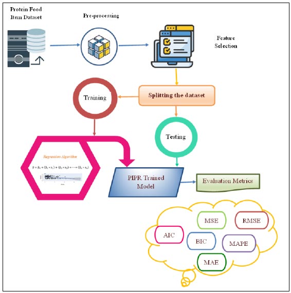
The PIPR model employs a regression algorithm to forecast protein-rich food items contributing to increased and decreased obesity, utilizing evaluation metrics as illustrated in Fig. (1). The process initiates with data preprocessing and feature selection to identify the most and least correlated variables. Subsequently, the dataset is partitioned into training and testing subsets. The model undergoes training through multiple iterations, and its performance is assessed using various metrics, ultimately demonstrating favorable results assessed by the adjusted R squared value. The model's validity is substantiated by AIC and BIC values concerning the testing data. Finally, evaluation metrics like MSE, RMSE, MAE, and MAPE are computed to predict the most and least correlated protein-rich food items.
2.3. Pre-processing - Feature Selection
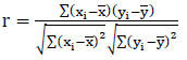
Real-world data often contains noise, missing values, or formats unsuitable for direct use in machine learning models. Data preprocessing becomes essential to clean and prepare the data for machine learning applications, thereby reducing errors and enhancing model effectiveness. In this particular model, the collected dataset undergoes preprocessing to manage missing data and assess correlation levels among attributes. Many machine learning models cannot handle missing values; hence, in this study, these missing values are substituted with mean values to address this issue. Once the missing values are replaced, feature selection techniques are applied to identify the most impactful features capable of enhancing model performance. Correlation analysis, specifically using methods like the Pearson Correlation Coefficient (PCC), is utilized for this research's feature selection process. The selected features demonstrate strong associations with the output variable while maintaining minimal associations among themselves. By employing independent-dependent variable correlations, this analysis identifies the variables exerting the most significant influence on an individual's obesity levels. The PCC is calculated using Eq. (1).
 (1)
(1)
In Eq. (1)
r denotes the Pearson Correlation Coefficient
xi and yi denotes the values of the x and y variables
(xi- ) - Variance of x
(xi- ) - Variance of y
and - Mean values of the variables x and y
 - Standard Deviation of x
 - Standard Deviation of y
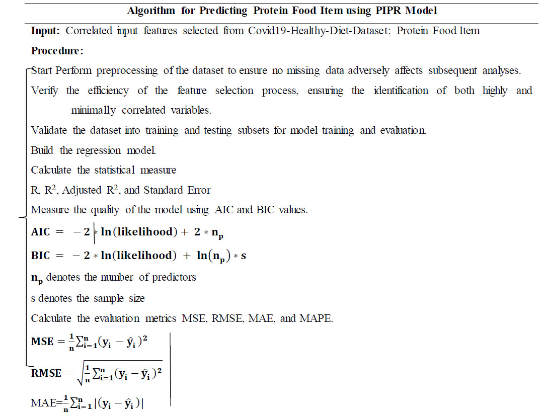
The algorithm for predicting protein food items is given below.
Algorithm for Predicting Protein Food Item using PIPR Model
| Most Correlated Variables | Least Correlated Variables | ||
|---|---|---|---|
| Name of the Variables | Correlation Value | Name of the Variables | Correlation Value |
| Animal products | 0.605 | Vegetal products | -0.369 |
| Meat | 0.592 | Cereals excluding beer | -0.390 |
| Milk including butter | 0.479 | Pulses | -0.451 |
| Eggs | 0.430 | Oilcrops | -0.605 |
| Vegetable oils | 0.364 | - | - |
In the correlation analysis conducted, the protein-rich food items most strongly associated with increased obesity are animal products, meat, milk (including butter), eggs, and vegetable oils. Conversely, the least closely correlated protein-rich food items linked to decreased obesity are vegetal products, cereals (excluding beer), pulses, and oil crops. Table 3 presents the correlation values corresponding to these most and least correlated protein food items.
A scatterplot serves to explore the connections between two variables, such as obesity and meat consumption. In a scatter plot, a positive association suggests that the variables increase or decrease simultaneously, while a negative association implies that if one variable increases, the other decreases, and vice versa. This study involves the analysis and development of machine learning models to predict obesity using highly and minimally associated protein food items. Figs. (2 and 3) depict scatter plots for these correlated variables, illustrating that as the consumption of protein-rich food items with the strongest correlation rises, so does the level of obesity, and conversely.
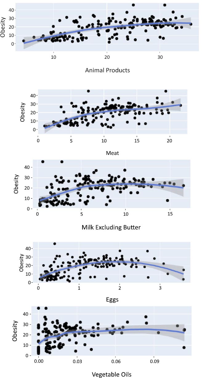
Scatter plot for the most correlated variables.
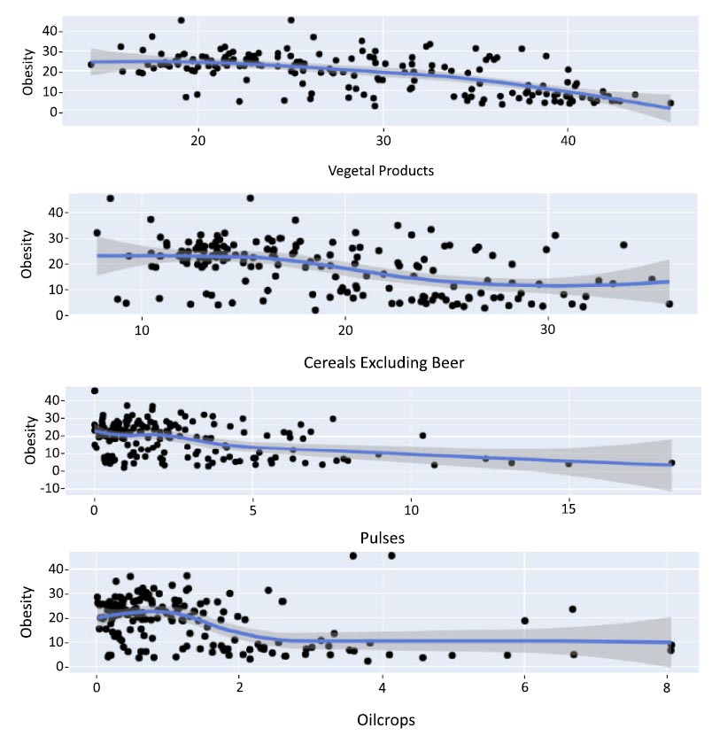
Scatter plot for the least correlated variables.
2.4. PIPR Machine Learning Model Development
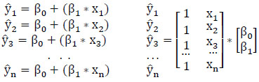
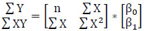
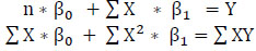
After feature selection, the dataset undergoes division into training data (80%) and testing data (20%) for the construction of the machine learning model. In order to construct a regression model, determination of the intercept (βo) and slope (β1) for each predictor variable is necessary. The proposed Protein Item Prediction Regression (PIPR) model utilizes Multiple Linear Regression (MLR) to forecast protein items influencing obesity, employing the regression equation derived from the Simple Linear Regression (SLR) Model represented in matrix form as (2).
 (2)
(2)
In (2), 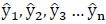 represent the predicted values generated by the model, where β 0 signifies the intercept, β1 represents the slope coefficient, and x1, x2, x3 ... xn denote the independent variables. These predicted values are collectively represented as a single-column (n×1) matrix Y.
The intercept and slope coefficients are also combined into a single (2, ×1) column vector.

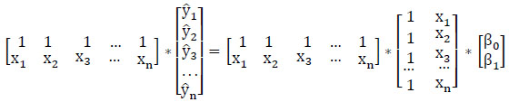
The values of the prediction variable are assembled into a (n × 2) matrix as depicted below.
Eq. (2) is rewritten as
 (3)
(3)
Eq. (3) is multiplied by XT on both sides to find the slope and intercept as given in (4).
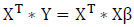 (4)
(4)
After multiplying with XT, (2) becomes
 (5)
(5)
After simplification, (5) becomes
(6)
 (7)
(7)
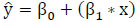
The elimination by substitution method is used to solve (7). After finding the intercept and slope, the model is fitted with a single predictor using (8).
(8)
The regression equation for MLR model uses several predictor variables to predict the outcome of a response variable. Extending (8) for several predictor variables, the regression equation for the MLR model is accomplished as given in (9).
 (9)
(9)
where β 0 denotes the intercept, β1, β2, β3, ... βn, denotes the slope coefficient, and x1, x2, x3, ... xn, denotes the predictor variables.
2.5. Regression Model for Most Correlated Variables
After the dataset splitting, this section encompasses the development of four MLR Models: MLR Model 1, MLR Model 2, MLR Model 3, and the PIPR Model, aimed at identifying the most correlated variables associated with increased obesity. Initially, the five most correlated protein items are utilized in MLR Model 1. Subsequently, based on the significance of the predictor variables, the least significant variable is eliminated, leading to the construction of MLR Model 2. This process continues by iteratively removing the least significant variable among the four most correlated protein items, forming subsequent models. The PIPR model created identifies the two most correlated protein items, both of which significantly impact the increase in obesity.
2.5.1. MLR Model 1
The MLR Model 1 identifies the most correlated protein food items using the prediction Eq. (10) to forecast obesity levels based on given values of protein food items. Table 4 displays the estimates, standard errors, t-values, and Pr(>|t|) for the protein-rich food items most correlated with obesity, including animal products, meat, milk (including butter), eggs, and vegetable oils. In Table 4, the Pr(>|t|) column denotes the p-value corresponding to the t-value presented. If the p-value is below a predetermined significance level (p = 0.05), the predictor variable is deemed to have a statistically significant association with the response variable in the model. Among the predictor variables, vegetable oils exhibit comparatively lower significance based on the Pr(>|t|) value compared to other variables. Consequently, an improved MLR Model 2 were constructed subsequent to the removal of the less statistically significant variable “vegetable oils”.
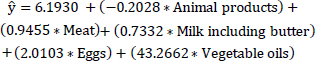 (10)
(10)
2.5.2. MLR Model 2
The refined regression model 2, focusing on the most correlated variables, is constructed following the elimination of the less statistically significant variable “vegetable oils”, as outlined in Eq. (11). Table 5 displays the estimates, standard errors, t-values, and Pr(>|t|) for the highly correlated variables-namely, animal products, eggs, meat, and milk (including butter)-after excluding the less statistically significant variable, “Vegetable Oils”. In the improved regression model 2, the predictor variable “animal products” exhibits lower significance based on the Pr(>|t|) compared to the other variables.
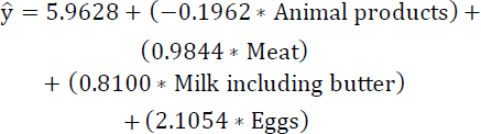 (11)
(11)
2.5.3. MLR Model 3
The refined regression model 3 is formulated for the most correlated variables subsequent to excluding the less statistically significant variable, “Animal products”, as expressed in Eq. (12). Table 6 presents the estimates, standard errors, t-values, and Pr(>|t|) for the highly correlated variables, specifically, meat, milk (including butter), and eggs after removing the less statistically significant variable, “Animal products”. In the improved regression model 3, the predictor variable “Eggs” demonstrates lower significance based on the Pr(>|t|) compared to the other variables.
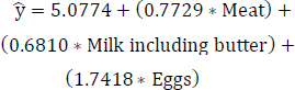 (12)
(12)
2.5.4. PIPR Model
The PIPR model focusing on the most correlated variables, subsequent to excluding the less statistically significant variable “Eggs”, is expressed in Eq. (13). Table 7 showcases the outcomes for the highly correlated variables-specifically, meat and milk (including butter)-after removing the less statistically significant variable “Eggs”. Finally, the protein-rich items “Meat” and “Milk including butter” exhibit greater statistical significance. These two items especially contribute to the increase of obesity levels, exerting a more substantial effect. The notable influence of these protein-rich items on obesity, as depicted in Fig. (4), highlights their potential as impactful contributors to the increase in obesity levels.
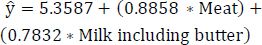 (13)
(13)
| Coefficients | Estimate | Std. Error | t value | Pr(>|t|) |
|---|---|---|---|---|
| Animal products | -0.2028 | 0.2252 | -0.9 | 0.036950 |
| Meat | 0.9455 | 0.2897 | 3.263 | 0.00140 ** |
| Milk including butter | 0.7332 | 0.2389 | 3.069 | 0.00261 ** |
| Eggs | 2.0103 | 1.0584 | 1.899 | 0.05970. |
| Vegetable oils | 43.2662 | 31.5874 | 1.37 | 0.17310 |
| Coefficients | Estimate | Std. Error | t value | Pr(>|t|) |
|---|---|---|---|---|
| Animal products | -0.1962 | 0.2259 | -0.869 | 0.386585 |
| Meat | 0.9844 | 0.2893 | 3.403 | 0.000881 *** |
| Milk including butter | 0.8100 | 0.2330 | 3.476 | 0.000688 *** |
| Eggs | 2.1054 | 1.0596 | 1.987 | 0.048979 * |
| Coefficients | Estimate | Std. Error | t value | Pr(>|t|) |
|---|---|---|---|---|
| Meat | 0.7729 | 0.1561 | 4.953 | 2.16e-06 *** |
| Milk including butter | 0.6810 | 0.1795 | 3.795 | 0.000223 *** |
| Eggs | 1.7418 | 0.9725 | 1.791 | 0.075551 |
| Coefficients | Estimate | Std. Error | t value | Pr(>|t|) |
|---|---|---|---|---|
| Meat | 0.8858 | 0.1439 | 6.155 | 8.03e-09 *** |
| Milk Including Butter | 0.7832 | 4.565 | 4.565 | 1.11e-05 *** |
Root cause for increased obesity.
2.6. Regression Model for Least Correlated Variables
Initially, four of the least correlated protein items among the 23 variables are inputted into MLR model 1. Subsequently, based on the significance of the predictor variables, the least significant variable is eliminated, leading to the creation of MLR model 2. This process continues iteratively for the three remaining least correlated protein items, removing the least significant variable each time. The PIPR model established identifies the two least correlated protein items, both of which play a significant role in reducing obesity.
2.6.1. MLR Model 1
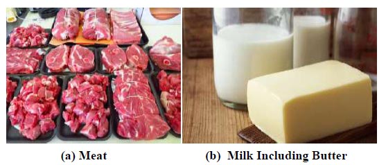
The MLR model 1 is constructed for the least correlated protein food items, employing a prediction equation that estimates obesity levels based on given values of vegetal products, cereals excluding beer, pulses, and oil crops, as presented in Eq. (14). Table 8 displays outputs such as estimates, standard errors, t-values, and Pr(>|t|) for these least correlated food items. Within Table 8, the predictor variable “cereals excluding beer” shows comparatively lower significance based on the Pr(>|t|) value in comparison to other variables. Subsequently, an improved regression model were established after eliminating the less statistically significant variable “cereals excluding beer”.
 (14)
(14)
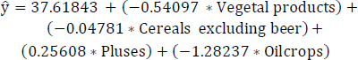
2.6.2. MLR Model 2
The refined regression MLR model 2 for the least correlated variables is formulated subsequent to eliminating the less statistically significant variable “cereals excluding beer”, depicted in Eq. (15). Table 9 presents the outputs, including estimates, standard errors, t-values, and Pr(>|t|), for the least correlated variables-namely, vegetal products, pulses, and oil crops-following the removal of the less statistically significant variable “cereals excluding beer”. In Table 9, the predictor variable “pulses” exhibits lower significance based on the Pr(>|t|) compared to the other variables. Consequently, an enhanced regression model is constructed after eliminating the statistically significant variable “pulses”.
 (15)
(15)
| Coefficients | Estimate | Std. Error | t value | Pr(>|t|) |
|---|---|---|---|---|
| Vegetal products | -0.54097 | 0.28882 | -1.873 | 0.0633 |
| Cereals excluding beer | -0.04781 | 0.27858 | -0.172 | 0.8640 |
| Pulses | -0.25608 | 0.39878 | -0.642 | 0.5219 |
| Oilcrops | -1.28237 | 0.53585 | -2.393 | 0.0181 * |
| Coefficients | Estimate | Std. Error | t value | Pr(>|t|) |
|---|---|---|---|---|
| Vegetal products | -0.5871 | 0.1052 | -5.581 | 1.28e-07 *** |
| Pulses | -0.2074 | 0.2790 | -0.743 | 0.45863 |
| Oilcrops | -1.2337 | 0.4529 | -2.724 | 0.00731 ** |
| Coefficients | Estimate | Std. Error | t value | Pr(>|t|) |
|---|---|---|---|---|
| Vegetal products | -0.63242 | 0.08559 | -7.389 | 1.39e-11 *** |
| Oil crops | -1.20439 | 0.45047 | -2.674 | 0.00843 ** |
Root cause for decreasing obesity.
2.6.3. PIPR Model
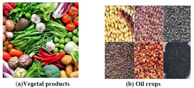
The PIPR model focusing on the least correlated variables, after the exclusion of the less statistically significant variable “pulses”, is represented in Eq. (16). Table 10 illustrates the estimates, standard errors, t-values, and Pr(>|t|) for the least correlated variables following the removal of the less statistically significant variable “pulses”. Remarkably, among these variables, “vegetal products” and “oil crops” exhibit more statistical significance. These two items particularly contribute to reducing obesity levels. Specifically, vegetables and oil crops emerge as high-impact potential protein-rich food items in the reduction of obesity, as highlighted in Fig. (5).
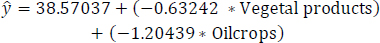 (16)
(16)
2.7. Regression Statistical Measure
The regression statistical measures provide insights into the model's performance. These measures encompass the correlation coefficient (R), the coefficient of determination (R2), the adjusted R-squared (Adjusted R2), and the standard error. The correlation coefficient (R) quantifies the strength of the relationship between two variables within the model. Meanwhile, the coefficient of determination (R2) serves as a goodness-of-fit metric, explaining how well the model fits the given data. The adjusted R-squared indicates the importance of a particular variable in the model. Additionally, the standard error is utilized to assess the accuracy of predictions made by the model. These regression statistical measures are employed on both the training and testing datasets to evaluate and understand the model's performance characteristics.
2.7.1. Correlation Coefficient (R)
The correlation coefficient (R) is a measure used to quantify the model's ability. Jacob Cohen (1992) proposed guidelines for interpreting correlation coefficients [22], which are presented in Table 11.
The R values for the most and least correlated variables are depicted in Tables 12 and 13, respectively. The values related to the most and least correlated variables in the testing data indicate a high R value for the PIPR MLR model.
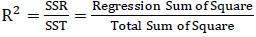
2.7.2. Coefficient of Determination (R2)
The R2 value ranges between 0 and 1. A high R2 suggests a well-fitted model for the data, while a low R2 indicates a poor fit or the absence of vital explanatory variables. However, a high R2 doesn't always guarantee an accurate model for estimation and forecasting; the assessment of fit relies on the analysis context. The coefficient of determination (R2) is calculated using Eq. (17). Especially, R2 tends to increase whenever an extra variable is included in the model, potentially leading to an artificially high R2 due to the inclusion of an excessive repressors. Tables 14 and 15 showcase the R2 values for the most and least correlated variables, respectively. It is observed that the R2 values for both the most and least correlated variables in both the training and testing data increase with the addition of an extra protein food item.
 (17)
(17)
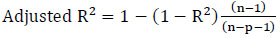
2.7.3. Adjusted R2
The adjusted R2 penalizes the inclusion of extra independent variables in the model. It increases only if a new independent variable enhances the model more than anticipated by chance. However, it decreases if a predictor improves the model by less than expected by chance. This value tends to penalize the adjusted R2 when an additionally added independent variable is ineffective, indicating that the variable has no effect on the dependent variable. Eq. (18) is used to calculate the adjusted R2. Tables 16 and 17 present the adjusted R2 values for the most and least correlated variables, respectively. In Table 16, concerning the most correlated variables in the training data, Model 1 demonstrates a high adjusted R2 value, while for the testing data, the PIPR model exhibits a high adjusted R2 value. In Table 17, for the least correlated variables in both the training and testing data, the adjusted R2 value is high for the PIPR model.
 (18)
(18)
| Correlation Coefficient Value | 0.0 to -0.30.0 to +0.3 | -0.5 to -0.30.3 to 0.5 | -0.9 to -0.50.5 to 0.9 | -1.0 to -0.90.9 to 1.0 |
|---|---|---|---|---|
| Association | Weak | Moderate | Strong | Very Strong |
| Name of the Model | Name of the Variables | MLR | |
|---|---|---|---|
| Training | Testing | ||
| R | R | ||
| PIPR | Meat+ Milk including butter | 0.815 | 0.854 |
| Model 3 | Eggs+ Meat+ Milk including butter | 0.806 | 0.812 |
| Model 2 | Animal products+ Eggs+ Meat+ Milk including butter | 0.800 | 0.808 |
| Model 1 | Vegetable oils + Animal products+ Eggs+ Meat+ Milk including butter | 0.789 | 0.799 |
| Name of the Model | Name of the Variables | MLR | |
|---|---|---|---|
| Training | Testing | ||
| R | R | ||
| PIPR | Oilcrops+ Vegetal products | 0.819 | 0.825 |
| Model 2 | Pulses+ Oilcrops+ Vegetal products | 0.811 | 0.818 |
| Model 1 | Cereals excluding beer + Pulses + Oilcrops+ Vegetal products | 0.801 | 0.812 |
| Regression Model | Name of the Variables | Training | Testing |
|---|---|---|---|
| R2 value | R2 value | ||
| PIPR | Meat+ Milk including butter | 0.903 | 0.943 |
| Model 3 | Eggs+ Meat+ Milk including butter | 0.827 | 0.830 |
| Model 2 | Animal products+ Eggs+ Meat+ Milk including butter | 0.810 | 0.814 |
| Model 1 | Vegetable oils + Animal products+ Eggs+ Meat+ Milk including butter | 0.802 | 0.810 |
| Regression Model | Name of the Variables | Training | Testing |
|---|---|---|---|
| R2 value | R2 value | ||
| PIPR | Oilcrops+ Vegetal products | 0.892 | 0.910 |
| Model 2 | Pulses+ Oilcrops+ Vegetal products | 0.899 | 0.913 |
| Model 1 | Cereals excluding beer + Pulses + Oilcrops+ Vegetal products | 0.902 | 0.920 |
Where p denotes the number of predictors, R2 denotes the coefficient of determination, and n represents the sample size.
| Regression Model | Name of the Variables | Training | Testing |
|---|---|---|---|
| Adjusted R2 value | Adjusted R2 value | ||
| PIPR | Meat+ Milk including butter | 0.912 | 0.921 |
| Model 3 | Eggs+ Meat+ Milk including butter | 0.839 | 0.845 |
| Model 2 | Animal products+ Eggs + Meat+ Milk including butter | 0.818 | 0.835 |
| Model 1 | Vegetable oils + Animal products+ Eggs+ Meat+ Milk including butter | 0.797 | 0.812 |
| Regression Model | Name of the variable | Training | Testing |
|---|---|---|---|
| Adjusted R2 value | Adjusted R2 value | ||
| PIPR | Oilcrops+ Vegetal products | 0.910 | 0.912 |
| Model 2 | Pulses+ Oilcrops+ Vegetal products | 0.895 | 0.881 |
| Model 1 | Cereals excluding beer + Pulses + Oilcrops+ Vegetal products | 0.855 | 0.878 |
| Regression Model | Name of the Variables | Training | Testing |
|---|---|---|---|
| Standard Error | Standard Error | ||
| PIPR | Meat+ Milk including butter | 7.331 | 6.911 |
| Model 3 | Eggs+ Meat+ Milk including butter | 7.271 | 6.955 |
| Model 2 | Animal products+ Eggs+ Meat+ Milk including butter | 7.278 | 6.948 |
| Model 1 | Vegetable oils + Animal products+ Eggs+ Meat+ Milk including butter | 7.254 | 6.992 |
| Regression Model | Name of the Variables | Training | Testing |
|---|---|---|---|
| Standard Error | Standard Error | ||
| PIPR | Oilcrops+ Vegetal products | 7.564 | 7.533 |
| Model 2 | Pulses+ Oilcrops+ Vegetal products | 7.536 | 7.671 |
| Model 1 | Cereals excluding beer + Pulses + Oilcrops+ Vegetal products | 7.524 | 7.797 |
| Regression Model | Name of the Variables | Testing | Testing |
|---|---|---|---|
| AIC | BIC | ||
| PIPR | Meat+ Milk including butter | 212.6744 | 218.4104 |
| Model 3 | Eggs+ Meat+ Milk including butter | 213.9378 | 221.1077 |
| Model 2 | Animal products+ Eggs+ Meat+ Milk including butter | 214.705 | 223.309 |
| Model 1 | Vegetable oils + Animal products+ Eggs+ Meat+ Milk including butter | 215.8803 | 225.9182 |
| Regression Model | Name of the variables | Testing | Testing |
|---|---|---|---|
| AIC | BIC | ||
| PIPR | Oilcrops+ Vegetal products | 218.0138 | 223.7498 |
| Model 2 | Pulses+ Oilcrops+ Vegetal products | 220.0116 | 227.1816 |
| Model 1 | Cereals excluding beer + Pulses + Oilcrops+ Vegetal products | 221.8572 | 230.4612 |
2.7.4. Standard Error (SE)
The standard error denotes the accuracy of predictions using the regression model. A smaller SE value indicates closer observations to the fitted line, while a larger SE value indicates observations farther away. The standard error values for the most and least correlated variables are displayed in Tables 18 and 19, respectively. In Table 18, the standard error values for the most correlated variables show low values in both the training and testing datasets. Regarding Table 19, for the least correlated variables, the standard error value is low in the training data for Model 1, and in the testing data, it is low for the PIPR model. The regression statistical measures support the quantification of the PIPR model's ability through the adjusted R2 value and standard error. Additionally, AIC and BIC are calculated to validate the model's quality.
2.8. PIPR Model Performance Evaluation
To ensure the proposed model's quality, the model's performance is assessed using two penalized likelihood criteria: Akaike Information Criterion (AIC) and Bayesian Information Criterion (BIC) concerning protein-rich food items. AIC penalizes the addition of extra variables to a model by imposing a penalty that increases the error as additional variables are included. Lower AIC values indicate a better model fit. On the other hand, BIC is a variation of AIC that imposes more penalty for incorporating extra variables. For model comparison, preference is given to the model exhibiting the lowest AIC and BIC scores. The AIC and BIC values for the most and least correlated variables are displayed in Tables 20 and 21, respectively. These values were computed using Eqs. (19 and 20), respectively.
 (19)
(19)
 (20)
(20)
Where np denotes the number of predictors, and s denotes the sample size.
3. RESULTS
3.1. Performance Metrics
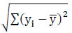
To create and implement a comprehensive model, it is essential to assess it using a variety of metrics. This process aids in improving the model's performance and refining it for better results. The proposed Protein Item Prediction Regression (PIPR) model for regression tasks employs various evaluation metrics, such as Mean Squared Error (MSE), Root Mean Squared Error (RMSE), Mean Absolute Percentage Error (MAPE), and Mean Absolute Error (MAE). MSE represents the squared difference between actual and predicted values, while RMSE calculates the average deviation between predicted and actual values. Lower values of MSE and RMSE indicate enhanced model accuracy. MAE measures the prediction error by determining the average absolute difference between the observed and predicted values. MAPE measures accuracy in terms of percentage by calculating the average absolute percent error between observed and actual values. Eqs. (21, 22, 23, and 24) are utilized to compute MSE, RMSE, MAE, and MAPE, respectively.
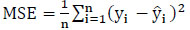 (21)
(21)
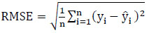 (22)
(22)
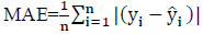 (23)
(23)
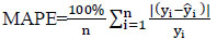 (24)
(24)
Where
n - Number of data points
yi - Observed values
 - Predicted values.
3.2. Performance Validation of the Proposed Model
The performance of the PIPR Model is validated by computing the performance metrics for the most and least correlated protein food items. The evaluation metric values for the most correlated variables, specifically meat and milk (without butter), within the PIPR model exhibit lower error values compared to other models, as illustrated in Table 22.
In the PIPR model, the evaluation metric values for the least correlated variables, namely, vegetal products and oil crops, display a lower error value of 7.24 compared to other models, as shown in Table 23, (Fig. 6).
| Regression Model | Name of the Variables | Testing Data | ||||
|---|---|---|---|---|---|---|
| MSE | RMSE | MAE | MAPE | |||
| PIPR | Meat+ Milk including butter | 49.59 | 7.04 | 5.08 | 29% | |
| Model 3 | Eggs+ Meat+ Milk including butter | 50.49 | 7.11 | 5.15 | 30% | |
| Model 2 | Animal products+ Eggs+ Meat+ Milk including butter | 51.05 | 7.15 | 5.31 | 34% | |
| Model 1 | Vegetable oils + Animal products+ Eggs+ Meat+ Milk including butter | 53.52 | 7.32 | 5.19 | 30% | |
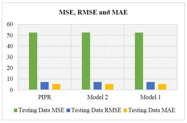
Model evaluation values for the least correlated variables.
| Regression Model | Name of the Variables | Testing Data | |||
|---|---|---|---|---|---|
| MSE | RMSE | MAE | MAPE | ||
| PIPR | Oilcrops + Vegetal products | 52.51 | 7.24 | 5.39 | 31% |
| Model 2 | Pulses+ Oilcrops+ Vegetal products | 52.57 | 7.25 | 5.40 | 32% |
| Model 1 | Cereals excluding beer +Pulses + Oilcrops Vegetal products | 52.47 | 7.24 | 5.39 | 32% |
4. DISCUSSION
In the regression model for the least correlated variables, Model 2's RMSE value is 7.25 and the MAE is 4.0, which includes vegetal products, oil crops, and pulses; however, Model 1's values are 7.24 and 5.34, respectively, which include vegetal products, cereals including beer, oil crops, and pulses; and the PIPR model's RMSE is 7.24 and the MAE is 5.39, which includes vegetal products and oil crops. Model 1 and the PIPR model have similar RMSE and MAE values, but the PIPR model has a lower MAPE value of 31% than Model 1. The statistical measure, adjusted R2 for the PIPR Model, is higher for testing data than the remaining three models for the most and least correlated protein food items. When compared with other models, the results of the evaluation metrics and statistical measures show that the proposed PIPR model for the most and least correlated protein food items has low error values and a high adjusted R2. This clearly shows that the model is the most efficient at predicting the protein food product with the greatest impact on obesity.
4.1. Proposed Method for the PIPR Model
4.1.1. Preprocessing
- Initially, the dataset undergoes preprocessing to handle missing data and assess correlation levels among attributes.
- Missing values are substituted with mean values to address this issue.
- Feature selection techniques are applied to identify the most impactful features capable of enhancing model performance.
4.1.2. Feature Selection
- Correlation analysis, specifically using methods like the Pearson Correlation Coefficient (PCC), is utilized for feature selection.
- The selected features demonstrate strong associations with the output variable while maintaining minimal associations among themselves.
- This analysis identifies the variables exerting the most significant influence on an individual's obesity levels.
4.1.3. Regression Model Development
- The dataset is partitioned into training and testing subsets.
- Multiple Linear Regression (MLR) models are developed for both the most correlated variables contributing to increased obesity and the least correlated variables reducing obesity.
- MLR models undergo iterative refinement, removing the least statistically significant variables among the correlated protein food items.
- The final PIPR model is formulated based on the most significant correlated variables identified through the iterative process.
4.1.4. Evaluation Metrics
- The model's predictive performance is assessed using various evaluation metrics, including Mean Squared Error (MSE), Root Mean Squared Error (RMSE), Mean Absolute Error (MAE), Mean Absolute Percentage Error (MAPE), adjusted R-squared, and standard error.
- Additionally, the model's quality is validated using penalized likelihood criteria such as Akaike Information Criterion (AIC) and Bayesian Information Criterion (BIC).
4.1.5. Final Ananlysis
- The PIPR model demonstrates its superiority in accurately predicting the impact of protein-rich foods on obesity, showcasing lower error rates and high adjusted R2 values across various metrics.
- Through rigorous evaluation, the proposed method offers valuable insights into the complex relationship between specific protein foods and obesity, positioning it as a promising tool for understanding and mitigating this global health concern.
CONCLUSION
Addressing the global health challenge of obesity requires proactive measures and comprehensive strategies. In this study, a novel approach, the Protein Food Item Prediction Regression (PIPR) model, was introduced and applied to forecast the influence of various protein-rich food items on obesity levels. Leveraging machine learning techniques and regression analysis, the PIPR model aimed to identify the protein foods most strongly associated with increased or decreased obesity. The research utilized a dataset encompassing information on diverse food types, global obesity and undernutrition rates, and COVID-19 cases across numerous countries. After rigorous preprocessing and feature selection techniques, the PIPR model underwent training and testing phases to assess its predictive capabilities. The findings from this study reveal significant insights into the correlation between specific protein-rich food items and obesity. Notably, the model identified certain protein foods that exhibit strong correlations with increased obesity, such as meat and milk (including butter). The PIPR model identified other protein-rich items, like vegetal products and oil crops, that showcased a more prominent link to reduced obesity rates. The performance evaluation metrics-Mean Squared Error (MSE), Root Mean Squared Error (RMSE), Mean Absolute Error (MAE), Mean Absolute Percentage Error (MAPE), adjusted R-squared, and standard error-consistently highlighted the PIPR model's superiority in predicting the impact of protein rich food items on obesity compared to alternative regression models. In summary, the PIPR model demonstrates promising efficiency in explaining the complex relationship between specific protein foods and obesity. Its ability to identify both positively and negatively correlated protein items with obesity emphasizes its potential in guiding dietary recommendations and public health policies aimed at combating obesity on a global scale. Further research and validation using diverse datasets and refined methodologies could enhance the model's precision and contribute significantly to mitigating the prevalence of obesity worldwide. Exploring the integration of longitudinal data and considering socio-economic factors could further enhance the predictive accuracy and practical utility of the model in addressing the complex dynamics of obesity.
AUTHORS' CONTRIBUTION
S. Vairachilai had done the methodology and writing.
S. Periyanayagi had done the implementation.
S.P. Raja had done drafting.
LIST OF ABBREVIATIONS
| PIPR | = Prediction Regression |
| LR | = Logistic Regression |
| NB | = Naive Bayes |
| ADA | = Adaptive Boosting |
| GB | = Gradient Boosting |
| BMI | = Body Mass Index |
| WC | = Waist Circumference |
| WHR | = Waist-hip Ratio |
| DT | = Decision Tree |
AVAILABILITY OF DATA AND MATERIALS
The data supporting the findings of the article is available in the [USDA (United States Department of Agriculture) Center for Nutrition Policy and Promotion recommends a daily diet] at https://www.kaggle.com/datasets/mariaren/Covid19-Healthy-Diet-Dataset, reference number [5].