All published articles of this journal are available on ScienceDirect.

Deep Learning based Feed Forward Neural Network Models for Hyperspectral Image Classification
Abstract
Introduction
Traditional feed-forward neural networks (FFNN) have been widely used in image processing, but their effectiveness can be limited. To address this, we develop two deep learning models based on FFNN: the deep backpropagation neural network classifier (DBPNN) and the deep radial basis function neural network classifier (DRBFNN), integrating convolutional layers for feature extraction.
Methods
We apply a training algorithm to the deep, dense layers of both classifiers, optimizing their layer structures for improved classification accuracy across various hyperspectral datasets. Testing is conducted on datasets including Indian Pine, University of Pavia, Kennedy Space Centre, and Salinas, validating the effectiveness of our approach in feature extraction and noise reduction.
Results
Our experiments demonstrate the superior performance of the DBPNN and DRBFNN classifiers compared to previous methods. We report enhanced classification accuracy, reduced mean square error, shorter training times, and fewer epochs required for convergence across all tested hyperspectral datasets.
Conclusion
The results underscore the efficacy of deep learning feed-forward classifiers in hyperspectral image processing. By leveraging convolutional layers, the DBPNN and DRBFNN models exhibit promising capabilities in feature extraction and noise reduction, surpassing the performance of conventional classifiers. These findings highlight the potential of our approach to advance hyperspectral image classification tasks.
1. INTRODUCTION
This article presents novel deep learning models with a feed-forward architecture and gradient descent learning designed for hyperspectral image classification [1]. The developed models, including the deep backpropagation neural network classifier (DBPNN) and deep radial basis function neural network classifier (DRBFNN), utilize convolutional layers for feature extraction. The training algorithm targets deep dense layers of both classifiers, aiming for effective classification with increased accuracy across hyperspectral datasets such as Indian Pine, University of Pavia, Kennedy Space Centre, and Salinas. The layer structures of DBPNN and DRBFNN are optimized for enhanced feature extraction and noise removal in hyperspectral images. Comprehensive training, rigorous testing, and meticulous validation are conducted on all four hyperspectral datasets, leading to the detailed reporting of their performance metrics. The evaluated metrics demonstrate the efficacy and accuracy of both deep learning feed-forward classifiers, showcasing their superiority in the classification process compared to existing classifiers [2].
A comprehensive advancement in image processing techniques is presented in this study, focusing on addressing feature loss in deep neural network-based algorithms. Employing a multi-level information compensation strategy and integrating the U-Net network architecture enhances image super-resolution recons truction, particularly in texture and edge details [3]. The Enhanced Image Inpainting Network employs a multi-scale feature module in conjunction with an enhanced attention mechanism, bolstering its ability to perform semantic image inpainting. Furthermore, the optimized loss function combines style and perceptual loss functions, thereby enhancing the model's overall performance [4]. The article introduces an innovative image inpainting algorithm utilizing a partial multi-scale channel attention mechanism and deep neural networks to address limitations in capturing multi-scale features with irregular defects [5]. Proposing an innovative approach to image restoration, this method integrates Semantic Priors, Deep Attention Residual Group, and Full-scale Skip Connection techniques. The Semantic Priors Network is tasked with learning comprehensive semantic information for missing regions, thereby facilitating precise completion. Meanwhile, the Deep Attention Residual Group concentrates on missing regions and adjusts channel features accordingly. Additionally, Full-scale Skip Connection merges low-level boundary information with high-level textures, enhancing the effectiveness of the restoration process [6]. A lightweight method is proposed, combining group convolution and attention mechanisms to enhance traditional convolution modules. Group convolution achieves multi-level image inpainting, while a rotating attention mechanism addresses information mobility between channels. A parallel discriminator structure ensures local and global consistency in the image inpainting process [7].
The paper addresses challenges in hyperspectral image classification using conventional methods, arising from the complexity of processing multiple spectral bands, hindering feature extraction and noise reduction. Traditional classifiers struggle with such data complexity. The article aims to leverage deep learning, especially feed-forward neural networks, to enhance classification accuracy, given their ability to autonomously learn features. It introduces two novel deep learning models- the deep backpropagation neural network classifier (DBPNN) and the deep radial basis function neural network classifier (DRBFNN)-tailored for hyperspectral image classification, incorporating convolutional layers for feature extraction. The goal is to improve feature extraction and noise reduction in hyperspectral images. By optimizing the layer structures of DBPNN and DRBFNN, the article aims to enhance classification accuracy across diverse hyperspectral datasets, ultimately overcoming traditional classifier limitations by leveraging deep learning for improved accuracy in feature extraction and noise reduction. Many prior studies in this domain exhibit deficiencies in their literature reviews, leading to a limited contextual understanding. Additionally, some suffer from methodological weaknesses, such as small sample sizes or inadequate controls, compromising the reliability of findings.
2. MATERIALS AND METHODS
2.1. Proposed Deep Learning-based FFNN Models
This work introduces two innovative deep learning models, a backpropagation neural network (DBPNN) and a radial basis function neural network (DRBFNN), designed for efficient hyperspectral image classification. Both classifiers leverage a structured layer design and employ the gradient descent learning rule for training. The incorporation of convolutional and pooling layers is specifically designed to extract crucial features from the input image datasets.
2.2. Developed Deep Learning-based Back-Propagation Neural Networks
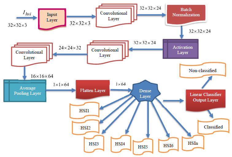
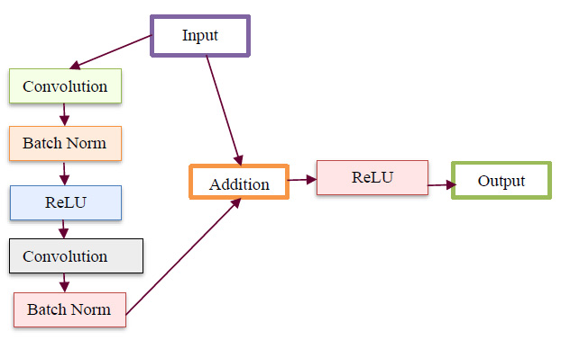
The newly modelled deep learning BPNN classifier comprises various layers, including input, convolutional, pooling, dense, flatten, and a linear classifier layer. The proposed DBPNN classifier is specifically designed to achieve enhanced training and learning performance, even in the presence of a limited dataset. This optimized deep learning BPNN model is employed for effective hyperspectral image classification, where the output from hyperspectral sensors serves as input for the DBPNN classifier, as illustrated in Fig. (1). A basic block diagram outlining the configuration of the input block is presented in Fig. (2).
2.2.1. Convolutional Layer
The proposed DBPNN classifier utilizes two-dimensional convolution layers during the training process to reduce the number of free parameters. These convolutional layers showcase the capacity of local receptive neurons and contribute to their weight update process [8]. Kernel filters within this layer regulate the input presented to the network model, involving a mathematical operation that employs the dot product of the kernel to diminish the filter matrix input.
 |
(1) |
 |
(2) |
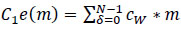
In this context, 'O' represents the two-dimensional output from the preceding layer, 'c' denotes the λ×λ kernel size matrix with learnable parameters used in the training process. The coordinates 'x' and 'y' cover all points of λ, while 'δ' signifies the location index in the two-dimensional kernel matrix. 'cw' denotes the kernel size of
a neuron, and the ‘*’ operator represents the cross-correlation operator. 'C1e(m)' refers to a one-dimensional convolution operation where the kernel movement is in one direction, although the input and output data pertain to a two-dimensional context. On the other hand, 'C2e(m)' signifies a two-dimensional convolution operation, where kernel positions extend in two directions, and three-dimensional input and output data are utilized. For this novel DBPNN classifier, only 'C2e(m)' operations are conducted, given that hyperspectral datasets correspond to image datasets, and 'C1e(m)' is used for time-series image operations in the convolution process [9].
2.2.2. Pooling Layer
In the proposed DBPNN classifier model, the designed pooling layer is connected to the successive convolutional layer, effectively reducing the spatial dimension of the extracted feature map. This pooling layer serves to mitigate overfitting issues. The mathematical represen- tation of the pooling operation is expressed as:
 |
(3) |
 |
(4) |
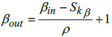
In this context, αin and βin represents the width and height of the input matrices, Skα denotes the height corresponding to the kernel size, specifies the width for the kernel size, αout and βout are the width and height of the output matrix, and ‘ρ’ denotes the stride factor during the pooling operation.
2.2.3. Activation Function
The DL-based back-propagation neural classifier utilizes a non-linear activation function to learn complex features from input datasets, particularly addressing the non-linearity in hyperspectral datasets. The classifier, designed with Rectified Linear Unit (ReLU) as the chosen non-linear activation function, enhances the overall performance of the deep learning model. Mathematically, ReLU is denoted as,
 |
(5) |
In Eq. (5), 'm' represents the input features of the image datasets.
2.2.4. Input and Dense Blocks
The input block initiates correlation between convolutional layers and progresses to deep dense blocks. Unlike traditional convolutional neural network models, this input block features a direct connection from input to output. This direct link is expressed as,
 |
(6) |
In this scenario, a parameter element matching factor is employed to match input and output segments, expressed as,
 |
(7) |
In this context, m represents the input to this block, μ signifies the output of these blocks, ξ denotes the mapping relationship between the input and output layer, and Dm represents the dimension matching factor.
Fig. (2) illustrates the internal structure of the input block from Fig. (1) in the deep BPNN model. This input block, receiving input image datasets, includes two convolutions, two batch normalizations, and one rectified linear unit block. The output from the batch normalization unit is added to the input, followed by another rectified linear unit and an output block. Progressing to the subsequent convolutional layer, the input block of the DBPNN model comprises 6 layers, while other architectural blocks contribute 8 layers, totaling 14 layers. Incorporating dropout, linear classification, softmax, and output layers, the model forms an 18-layer Deep Back Propagation Neural Network. Notably, the developed deep BPNN model outperforms traditional convolutional layer networks, demonstrating increased accuracy with deeper network depths compared to CNN models.
2.2.5. Classification Layer
In the proposed DBPNN model, the classification layer is designed with the 'softmax' function and a fully connected (FC) layer. The fully connected layer interconnects neurons between layers, forming a dense layer with correlated perception neurons, expressed as,
 |
(8) |
Eq. (8), ω0 represents the bias, and the ultimate output generated by the DBPNN model is denoted as ‘μ’. The novel DBPNN classifier aims to capture hyperspectral sensor images, effectively classifying them based on boundaries and performing precise segmentation.
2.2.6. Batch Normalization
In the new DBPNN classifier, the training image dataset is divided into dissimilar mini-batches for batch normalization, optimizing computational burden, and convergence. The initial normalization involves scaling the input image datasets, and subsequent activations enhance training speed, stability, and consistency. The architectural design in Fig. (1) aims to eliminate noise from captured hyperspectral sensor images, extract significant features using convolutional layers, and address lower gradient features with the dropout layer. This process enhances the effectiveness of hyperspectral image classification in the new DBPNN classifier.
2.3. Novel Deep Learning-Based Radial Basis Function Neural Networks
The multi-layer feedforward radial basis function neural model, utilized the Gaussian activation function for determining the final network output. In the architectural design of the multi-layer RBFNN, the norm is computed by adding the norm (ϕ) with the functional layer of the basic RBFNN model. The function representing the connection link between the hidden and output layers is expressed as,
 |
(9) |
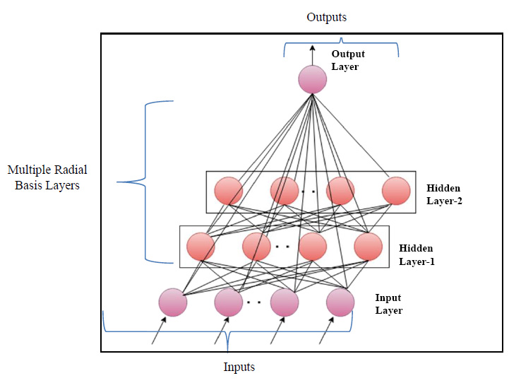
In Eq. (9), 'x' denotes the input data, 'α' is the learning rate, 'w' represents connective link weights, 'N' stands for the number of data samples, and 'Ri' indicates the radius of neighborhood pixels for computing the Euclidean distance norm. The Gaussian activation function is applied to each radial basis function neuron to obtain the final network output. Fig. (3) illustrates the architecture of the conventional RBF neural network model. The multi-layer equations defining the radial basis function are provided as follows:
 |
(10) |
 |
(11) |
 |
(12) |
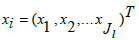
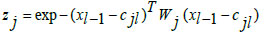
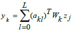
In Eqs. (10-12), 'xi,' 'zj,' and 'yk' represent the input neuronal output, hidden radial basis layer output, and the final output from the output layer, respectively. Eq. (11) features the weight matrix 'Wj' and center vector 'cjl,' while in Eq. (12), 'akl' indicates the coefficient vector of the output layer, 'Wk' defines the weight matrix between the hidden and output layers with 'zj' as the output from the hidden layer. The RBF model's final output is determined by the linear combination of all basis layers across the entire network.
2.3.1. Modelling the New DRBFNN Classifier Model
The deep learning-based radial basis function classifier is structured for non-linear transformations in the deep hidden layers. It operates through pre-training and fine-tuning, utilizing an auto-encoder for pre-training and back-propagation with gradient descent for fine-tuning. The auto-encoder's design involves an encoder mapping high-dimensional data to low-dimensional data and a decoder reconstructing the encoded information. The encoded data is represented as,
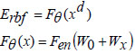 |
(13) |
In this context, ‘Fθ’ represents the encoder function, ‘xd’ denotes the datasets, ‘W0’ indicates the bias, and ‘Wx’ specifies the weight values. The reconstructed dataset by the decoder is obtained as,
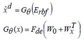 |
(14) |
In Eqs. (13 and 14), Fen and Fde represent the encoding activation and decoding activation, respectively, with ‘W0’ as the bias entity and ‘Wx’ as the weight entity. The new Deep Radial Basis Function Neural Network is structured to minimize the reconstruction error concerning the training data samples. The cost function calculates the difference between the encoded and decoded data samples, and the reconstruction error metric is assessed as,
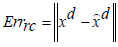 |
(15) |
The cost function defined for minimization of the reconstruction error is given by,
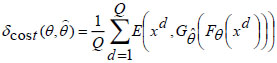 |
(16) |
During pre-training, all ‘Q’ auto-encoders from the preceding deep layers are consolidated, and the encoding operation for the input samples is carried out at both the input layer and the initial deep layer of the proposed DRBFNN classifier. The training of the new DRBFNN, incorporating its training parameters and the encoded dataset, is represented as,
 |
(17) |
Using the input xd, the combination of the input layer and the first deep layer in the DRBFNN classifier serves as the encoder neural network for the initial auto-encoding process. As the first auto-encoder begins its training, minimizing the reconstruction error, the initial training parameter set initializes the first deep layer of the DRBFNN, resulting in the final Qth-encoded vector.
 |
(18) |
In Eq. (18), ‘θQ’ represents the Q-th trained parameters of the DRBFNN encoder module. Through the described operations, each deep layer of the new DRBFNN classifier undergoes pre-training with Q-stacked auto-encoders to enhance learning and generalization abilities. Subsequently, fine-tuning is executed using the back-propagation algorithm, culminating in the final output from the developed DRBFNN model.
 |
(19) |
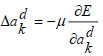
The output parameter is denoted as ‘θQ+1’. The error metric assessed throughout the training process is defined as,
 |
(20) |
With,  and it is updated using,
 |
(21) |
In Eq. (21), ‘α’ indicates the learning rate of the training process.
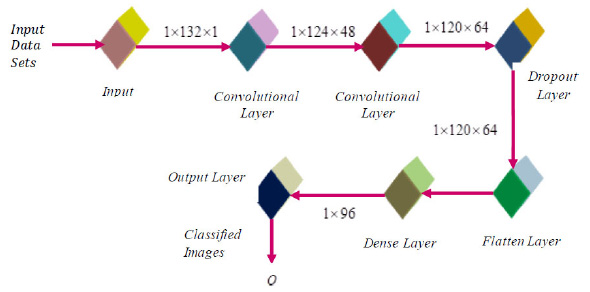
The new DRBFNN classifier is utilized for hyperspectral image classification, focusing on automatic feature detection without human intervention or additional feature extraction techniques. This deep learning-based RBFNN model effectively learns significant features for respective classes through convolution and pooling operations. The DRBFNN's architecture includes input, convolutional, dense, dropout, and output layers. Input images, sized [1×132×1], maintain their dimensionality through the convolutional layer. With two convolutional layers, the output progresses from [1×132×1] to [1×120×64]. Flattening yields were [1×7680], followed by dropout and a dense layer, reducing the size to [1×96]. The output layer classifies the entire dataset, recognizing hyperspectral features. Fig. (4) depicts the proposed deep learning-based radial basis function neural network architecture.

2.3.2. Convolution (Conv)
Each layer is linked to the subsequent layers through weight parameters along connection links, forming filters convoluted with the input layer. These filters slide over local receptive fields in the input datasets, acting as feature detectors and generating feature maps. The output of the convolutional layer is expressed as,
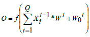 |
(22) |
where, ‘f’ represents the activation function, is the weight parameters, indicates the bias of the present layer with representing the input from the earlier layer.
2.3.3. Activation Function
Activating to determine the network model's output, this layer executes non-linear transformations for image class discrimination based on the output from the convolutional filter.
2.3.4. Pooling Layer
The convolutional layer produces a feature map, which undergoes subsampling at the pooling layer, resulting in,
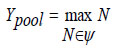 |
(23) |
In Eq. (23), 'ψ' denotes the pooling size. Compared to other classifiers, the newly developed Deep Learning-based RBFNN, featuring multiple hidden dense layers representing complex functions, exhibits improved learning and generalization abilities. Refer to Fig. (5) for the flowchart of the proposed DRBFNN classifier algorithm. The algorithmic steps for hyperspectral image classification using the deep learning radial basis function classifier are as follows:
2.3.5. Algorithm: DRBFNN_Classifier_Training
Input: hyperspectral_images, DRBFNN_classifier_ parameters, architectural_layers
Output: trained_DRBFNN_classifier, output_layer_ dimension, MSE_value
Step 1: Initialize DRBFNN_classifier_parameters, architectural_ layers
Step 2: Input hyperspectral_images to neural_ network_input_layer
Step 3: Configure_classifier_layers(Q)
Step 4: for i = 1 to Q do
Set_parameters_for_i-th_deep_hidden_layers
Step 5: Test if parameters for all deep layers are initially set:
If yes, proceed to Step 6
If no, return to Step 3
Step 6: Evaluate_output_layer_dimension()
Step 7: Execute_training_trial()
Step 8: Assess_MSE_value()
Step 9: Update_network_weights()
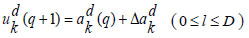 |
(24) |
 |
(25) |
 |
(26) |
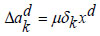 |
(27) |
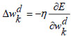 |
(28) |
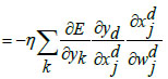 |
(29) |
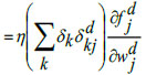 |
(30) |
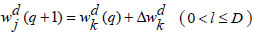
The last dense layer weights is updated by the following equations:
 |
(31) |
 |
(32) |
Step 10: Check for stopping condition:
If minimal MSE value and improved classification accuracy rate achieved:
Halt process and return classified_images
Else:
Repeat procedures from Step 6.
3. HYPERSPECTRAL IMAGE DATASETS
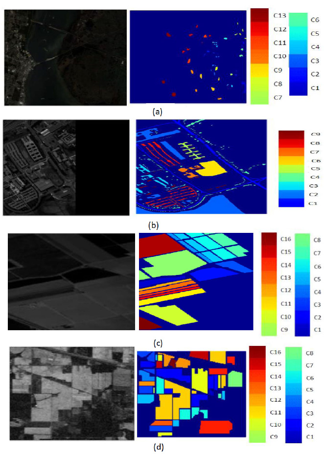
This study utilizes four distinct hyperspectral image datasets to evaluate the efficacy of the novel DBPNN and DRBFNN classifiers [10]. Fig. (6) illustrates the hyperspectral bands and ground truth information of the dataset. These datasets consist of the Kennedy Space Centre datasets, University of Pavia datasets, Salinas datasets, and Indian Pine datasets. A detailed presentation of each dataset is provided below:
3.1. Kennedy Space Centre (KSC) Datasets
These datasets were captured in 1996 by NASA in Florida, USA, using wavelengths ranging from 400 to 2500nm and 224 bands. After excluding water-absorbed entities, 176 bands were utilized for the study. The dataset encompasses 13 classes representing various land-covered areas (Table 1), and Fig. (6a) depicts the ground truth.
3.2. University of Pavia Datasets
These datasets were acquired from an urban area in North Italy, employing a reflective optics spectrographic image sensor. Furthermore, this dataset comprises 103 hyperspectral bands, with each image at a resolution of 610x340 pixels and a 1.3m spatial resolution, and is categorized into 9 classes (Table 2). Fig. (6b) provides the ground truth information.
| Labelled Classes | Class Category | Total Samples | Labelled Classes | Class Category | Total Samples |
|---|---|---|---|---|---|
| C1 | Scrub | 761 | C8 | Graminoid marsh | 431 |
| C2 | Willow swamp | 243 | C9 | Spartina marsh | 520 |
| C3 | Cabbage palm hammock | 256 | C10 | Cattail marsh | 404 |
| C4 | Cabbage palm/oak hammock | 252 | C11 | Salt marsh | 419 |
| C5 | Slash pine | 161 | C12 | Mud flats | 503 |
| C6 | Oak/broadleaf hammock | 229 | C13 | Water | 927 |
| C7 | Hardwood swamp | 105 | |||
| Total Data samples of KSC dataset | 5211 | ||||
| Labelled Classes | Class Category | Total Samples | Labelled Classes | Class Category | Total Samples |
|---|---|---|---|---|---|
| C1 | Asphalt | 6631 | C6 | Bare soil | 5029 |
| C2 | Meadows | 18649 | C7 | Bitumen | 1330 |
| C3 | Gravel | 2099 | C8 | Self-blocking bricks | 3682 |
| C4 | Trees | 3064 | C9 | Shadows | 947 |
| C5 | Painted metal sheets | 1345 | |||
| Total Data samples of Pavia dataset | 42776 | ||||
| Labelled Classes | Class Category | Total Samples | Labelled Classes | Class Category | Total Samples |
|---|---|---|---|---|---|
| C1 | Brocoli green weeds 1 | 2009 | C9 | Soil vineyard | 6203 |
| C2 | Brocoli green weeds 2 | 3726 | C10 | Corn senesced green weeds | 3278 |
| C3 | Fallow | 1976 | C11 | Lettuce romaine 4wk | 1068 |
| C4 | Fallow rough plow | 1394 | C12 | Lettuce romaine 5wk | 1927 |
| C5 | Fallow smooth | 2678 | C13 | Lettuce romaine 6wk | 916 |
| C6 | Stubble | 3959 | C14 | Lettuce romaine 7wk | 1070 |
| C7 | Celery | 3579 | C15 | Vinyard untrained | 7268 |
| C8 | Grapes untrained | 11271 | C16 | Vinyard vertical trellis | 1807 |
| Total Data samples of Salinas dataset | 54129 | ||||
| Labelled Classes | Class Category | Total Samples | Labelled Classes | Class Category | Total Samples |
|---|---|---|---|---|---|
| C1 | Alfalfa | 46 | C9 | Oats | 20 |
| C2 | Corn-notill | 1428 | C10 | Soybean-notill | 972 |
| C3 | Corn-mintill | 830 | C11 | Soybean-mintill | 2455 |
| C4 | Corn | 237 | C12 | Soybean-clean | 593 |
| C5 | Grass-pasture | 483 | C13 | Wheat | 205 |
| C6 | Grass-trees | 730 | C14 | Woods | 1265 |
| C7 | Grass-pasture-mowed | 28 | C15 | Buildings-Grass-Trees-Drives | 386 |
| C8 | Hay-windrowed | 478 | C16 | Stone-Steel-Towers | 93 |
| Total Data samples of Indian Pine dataset | 10249 | ||||
3.3. Salinas Datasets
These datasets were captured using an AVIRIS sensor with a 3.7m spatial resolution over the Salinas Valley, California, USA. Additionally, it encompasses 217 samples, excluding 20 water absorption bands. The ground truth includes 16 classes, such as bare soils, vegetables, and vineyard fields (Table 3). Fig. (6c) illustrates the ground truth.
3.4. Indian Pine Datasets
These datasets were captured from Northwestern Indiana using an AVIRIS sensor with 145 pixels, 224 spectral bands, and wavelengths ranging from 0.4 to 2.5 x 10⁻⁶ m. Moreover, this dataset is categorized into 16 classes, with bands reduced to 200 after eliminating water-absorbed areas [11]. The dataset comprises 10249 data samples, including vegetation, forest, agriculture, dual lanes for rail lanes, housing, and built structures with roads (Table 4). Fig. (6d) presents the ground truth information [12].
These hyperspectral image datasets exhibit distinct features and notable differences among them. Key distinctions include the use of various sensors, absolute variability in ground truth data due to diverse geographical locations, differences in spatial resolution and spectral bands for each dataset, and varying labeled classes (13, 9, 16, and 16 for KSC, University of Pavia, Salinas’s dataset, and Indian Pines dataset respectively) [13]. Additionally, ground sample distances differ for each dataset (18m, 1.3m, 3.7m, and 20m).
To demonstrate the effectiveness of the proposed DBPNN and DRBFNN classifier model, it undergoes training, testing, and validation across all these datasets, each possessing its unique features. In the data distribution, 70% of samples are allocated for training, with the remaining 30% are reserved for testing [14]. To optimize training metrics, the number of training samples exceeds that of testing samples. The error criterion, represented by Eq. (20), is evaluated for both DBPNN and DRBFNN classifiers, aiming to minimize errors during their run [15].
4. RESULTS AND DISCUSSIONS
The proposed DBPNN and DRBFNN classifiers are simulated and validated to demonstrate their efficacy for the hyperspectral image datasets outlined in Section 1.5. Both models utilize deep learning with back-propagation and radial basis functions, employing gradient descent learning with distinct activation functions. The DBPNN classifier comprises 9 layers, including input, 7 deep hidden layers (convolutional, pooling, flatten, dense, dropout, and classification), and output. In contrast, the new DRBFNN classifier features 7 layers, encompassing input, 5 deep hidden layers, and output, each incorporating convolutional, pooling, flatten, dense, dropout, and classification components. This deep learning mechanism enhances classifier learning for improved classification outcomes.
The devised classifier model, encompassing DBPNN and DRBFNN, processes image data samples from the four hyperspectral datasets: KSC, University of Pavia, Salinas, and Indian Pine. The output neurons in the final layer match the number of classes (13, 9, 16, and 16 for the respective datasets). Detecting the correct class improves classification metrics, while iterative updates minimize errors and enhance accuracy. Training, testing, and validation occur in MATLAB R2021a, and the results, along with various parameters (Table 5), are reported. Both DBPNN and DRBFNN classifiers employ gradient descent learning with diverse activation functions, iteratively updating weighted interconnections to minimize Mean Square Error (Errormse) per Eq. (20).
| Classifier Metrics | DBPNN Metric Values | DRBFNN Metric Values |
|---|---|---|
| Learning rate | 0.2 | 0.2 |
| Learning approach | Deep learning | Deep learning |
| Learning rule | Gradient Descent learning | Gradient Descent learning |
| Activation function | Bipolar Tangential sigmoidal activation | Gaussian activation function |
| Convolutional Layers | 3 | 2 |
| Pooling layers | 1 | 1 |
| Dense layers | 2 | 2 |
| No. of epochs | Until error convergence | Until error convergence |
| No. of trials | 32 | 32 |
| Layer structure | 1-7-1 (Input layer -deep layers-Output layer) | 1-5-1 (Input layer -deep layers-Output layer) |
| Error convergence | 10-6 | 10-6 |
| Classification Accuracy (Acccl) | |||||||
|---|---|---|---|---|---|---|---|
| Kennedy Space Centre Datasets | University of Pavia Datasets | ||||||
| Labelled Classes | Class Category |
Proposed DBPNN classifier model |
Proposed DRBFNN classifier Model |
Labelled Classes |
Class Category |
Proposed DBPNN classifier model |
Proposed DRBFNN classifier Model |
| C1 | Scrub | 96.88 | 96.88 | C1 | Asphalt | 97.65 | 97.91 |
| C2 | Willow swamp | 97.45 | 97.53 | C2 | Meadows | 97.02 | 97.69 |
| C3 | Cabbage palm hammock | 96.99 | 97.82 | C3 | Gravel | 96.99 | 97.38 |
| C4 | Cabbage palm/oak hammock | 97.32 | 98.69 | C4 | Trees | 96.35 | 98.17 |
| C5 | Slash pine | 97.44 | 98.47 | C5 | Painted metal sheets | 97.68 | 98.47 |
| C6 | Oak/broadleaf hammock | 97.99 | 98.02 | C6 | Bare soil | 97.31 | 98.56 |
| C7 | Hardwood swamp | 97.67 | 97.84 | C7 | Bitumen | 97.85 | 98.34 |
| C8 | Graminoid marsh | 97.81 | 98.14 | C8 | Self-blocking bricks | 96.83 | 97.84 |
| C9 | Spartina marsh | 96.93 | 97.37 | C9 | Shadows | 97.54 | 97.98 |
| C10 | Cattail marsh | 97.28 | 97.93 | ||||
| C11 | Salt marsh | 97.55 | 98.00 | ||||
| C12 | Mud flats | 97.39 | 97.98 | ||||
| C13 | Water | 97.24 | 98.26 | ||||
Tables 6 and 7 present the computed classification accuracy for the proposed DBPNN and DRBFNN classifiers across hyperspectral image datasets (KSC, University of Pavia, Salinas, and Indian Pine). Table 6 focuses on KSC and Pavia datasets, revealing that, for KSC, DRBFNN consistently outperforms DBPNN, achieving accuracy rates exceeding 97.5% for classes C6, C8, and C7. Notably, C4, C5, and C13 exhibit prominent accuracy rates of 98.69%, 98.47%, and 98.26%, respectively. Similarly, for the University of Pavia datasets, DRBFNN surpasses DBPNN across all labelled classes, with C7 at 97.85%, C5 at 97.68%, and C1 at 97.65%, achieving overall accuracy higher than 96%. In both KSC and Pavia datasets, the superiority of DRBFNN over Deep BPNN is evident, attributed to the Gaussian activation function. Specifically, for Pavia's C6, DRBFNN achieves a notable 98.56% accuracy. The deep radial basis function classifier consistently demonstrates superior classification for labelled classes in both datasets.
| Classification Accuracy (Acccl) | |||||||
|---|---|---|---|---|---|---|---|
| Salinas Datasets | Indian Pines Dataset | ||||||
| Labelled Classes | Class Category |
Proposed DBPNN classifier model |
Proposed DRBFNN classifier model |
Labelled Classes | Class Category |
Proposed DBPNN classifier model |
Proposed DRBFNN classifier model |
| C1 | Brocoli green weeds 1 | 97.33 | 98.77 | C1 | Alfalfa | 97.84 | 98.65 |
| C2 | Brocoli green weeds 2 | 97.59 | 98.64 | C2 | Corn-notill | 98.03 | 98.04 |
| C3 | Fallow | 96.88 | 98.31 | C3 | Corn-mintill | 96.98 | 98.67 |
| C4 | Fallow rough plow | 97.41 | 98.49 | C4 | Corn | 97.15 | 98.48 |
| C5 | Fallow smooth | 97.96 | 98.68 | C5 | Grass-pasture | 96.41 | 97.96 |
| C6 | Stubble | 96.88 | 98.69 | C6 | Grass-trees | 98.84 | 98.61 |
| C7 | Celery | 97.43 | 97.85 | C7 | Grass-pasture-mowed | 97.63 | 97.51 |
| C8 | Grapes untrained | 97.67 | 98.95 | C8 | Hay-windrowed | 97.54 | 98.60 |
| C9 | Soil vineyard | 96.85 | 98.86 | C9 | Oats | 96.81 | 98.74 |
| C10 | Corn senesced green weeds | 96.79 | 98.78 | C10 | Soybean-notill | 98.77 | 97.95 |
| C11 | Lettuce romaine 4wk | 97.38 | 98.81 | C11 | Soybean-mintill | 98.05 | 97.99 |
| C12 | Lettuce romaine 5wk | 97.59 | 98.88 | C12 | Soybean-clean | 97.48 | 98.47 |
| C13 | Lettuce romaine 6wk | 97.81 | 98.98 | C13 | Wheat | 97.66 | 98.61 |
| C14 | Lettuce romaine 7wk | 97.40 | 98.69 | C14 | Woods | 96.89 | 97.91 |
| C15 | Vinyard untrained | 97.29 | 98.96 | C15 | Buildings-Grass-Trees-Drives | 97.84 | 98.04 |
| C16 | Vinyard vertical trellis | 98.14 | 98.75 | C16 | Stone-Steel-Towers | 98.75 | 98.18 |
| Mean Square Error (Errormse) | |||||||
|---|---|---|---|---|---|---|---|
| Kennedy Space Centre Datasets | University of Pavia Datasets | ||||||
| Labelled Classes | Class Category |
Proposed DBPNN classifier model |
Proposed DRBFNN classifier model |
Labelled Classes | Class Category |
Proposed DBPNN classifier model |
Proposed DRBFNN classifier Model |
| C1 | Scrub | 0.0716 | 0.0526 | C1 | Asphalt | 0.0618 | 0.0315 |
| C2 | Willow swamp | 0.0627 | 0.0319 | C2 | Meadows | 0.0073 | 0.0054 |
| C3 | Cabbage palm hammock | 0.0865 | 0.0718 | C3 | Gravel | 0.0196 | 0.0059 |
| C4 | Cabbage palm/oak hammock | 0.0540 | 0.0112 | C4 | Trees | 0.0095 | 0.0087 |
| C5 | Slash pine | 0.0641 | 0.0102 | C5 | Painted metal sheets | 0.0078 | 0.0042 |
| C6 | Oak/broadleaf hammock | 0.0927 | 0.0905 | C6 | Bare soil | 0.0036 | 0.0019 |
| C7 | Hardwood swamp | 0.0681 | 0.0098 | C7 | Bitumen | 0.00039 | 0.00018 |
| C8 | Graminoid marsh | 0.0731 | 0.0694 | C8 | Self-blocking bricks | 0.0027 | 0.0011 |
| C9 | Spartina marsh | 0.0548 | 0.0219 | C9 | Shadows | 0.00069 | 0.00046 |
| C10 | Cattail marsh | 0.0578 | 0.0369 | ||||
| C11 | Salt marsh | 0.0621 | 0.0199 | ||||
| C12 | Mud flats | 0.0692 | 0.0072 | ||||
| C13 | Water | 0.0573 | 0.0186 | ||||
Table 7 displays computed classification accuracy results for Salinas and Indian Pine datasets using the proposed classifiers. On average, the DBPNN and DRBFNN classifiers achieve 97.40% and 98.69% accuracy for Salinas. Notably, DBPNN is most effective for classes C16 (98.14%) and C5 (97.96%) in Salinas. DRBFNN achieves over 98% accuracy for all Salinas class labels, with 97.85% for celery. For Indian Pines, DBPNN and DRBFNN reach mean accuracies of 97.67% and 98.27%, respectively. DBPNN excels for labels C1, C6, C10, C11, and C16 (>98% accuracy). DRBFNN outperforms for C1-C4, C6, C8-C9, C12-C13, C15-C16. Overall, DRBFNN consistently outperforms DBPNN in both Tables 6 and 7, attributed to the Gaussian radial basis activation function with regularization ability.
The classifier underwent training and testing for a specified number of epochs to achieve minimal mean square error, aiming to minimize the error defined in Eq. (20). Tables 8 and 9 show the evaluated mean square error (Errormse) during classifier simulation for the four hyperspectral image datasets. In Table 8, the proposed DBPNN and DRBFNN classifiers achieve average mean square errors of 0.0672 and 0.0347 for the KSC datasets and 0.0126 and 0.00659 for the University of Pavia datasets, respectively. Notably, for both datasets, the new deep radial basis function neural network classifier attains a lower MSE value than the deep back-propagation neural network model. For the Salinas and Indian Pine datasets, the average Errormse is 0.0571 and 0.02334, and 0.040775 and 0.03145, respectively, using the DBPNN and DRBFNN classifier models. The convergence of error values validates the effectiveness of the proposed classifier models, with the DRBFNN classifier demonstrating superiority in hyperspectral image classification compared to the DBPNN classifier.
Fig. (7) illustrates image classification for KSC datasets using the proposed deep learning-based back propagation neural network model and radial basis function neural network model. In Fig. (7a and b), showcase the false color image and RGB image, respectively. Classification outcomes for KSC datasets, employing 3DMWCNN [16], GF+CNN [17], DW-SDA [18], MMS [19], GFO [20], PCA+SSA Classifier [21], DBPNN, and DRBFNN, are presented in Fig. (7c to j). The DRBFNN classifier demonstrates superior classification accuracy for KSC datasets, as evident in Fig. (7j). The unique and superior results achieved with the new classifier are confirmed by the distinctly classified image based on labeled classes.
| Mean Square Error (Errormse) | |||||||
|---|---|---|---|---|---|---|---|
| Salinas Datasets | Indian Pine Datasets | ||||||
| Labelled Classes | Class Category | Proposed DBPNN Classifier Model | Proposed DRBFNN Classifier Model | Labelled Classes | Class Category | Proposed DBPNN Classifier Model | Proposed DRBFNN Classifier Model |
| C1 | Brocoli green weeds 1 | 0.0723 | 0.0664 | C1 | Alfalfa | 0.0945 | 0.0823 |
| C2 | Brocoli green weeds 2 | 0.0852 | 0.0048 | C2 | Corn-notill | 0.0761 | 0.0562 |
| C3 | Fallow | 0.0104 | 0.0092 | C3 | Corn-mintill | 0.0349 | 0.0126 |
| C4 | Fallow rough plow | 0.0617 | 0.0129 | C4 | Corn | 0.0107 | 0.0085 |
| C5 | Fallow smooth | 0.1029 | 0.0083 | C5 | Grass-pasture | 0.0912 | 0.0827 |
| C6 | Stubble | 0.0713 | 0.0627 | C6 | Grass-trees | 0.0768 | 0.0603 |
| C7 | Celery | 0.1249 | 0.0087 | C7 | Grass-pasture-mowed | 0.0066 | 0.0051 |
| C8 | Grapes untrained | 0.0922 | 0.0256 | C8 | Hay-windrowed | 0.0309 | 0.0265 |
| C9 | Soil vineyard | 0.0602 | 0.0687 | C9 | Oats | 0.0511 | 0.0428 |
| C10 | Corn senesced green weeds | 0.0105 | 0.0083 | C10 | Soybean-notill | 0.0104 | 0.0096 |
| C11 | Lettuce romaine 4wk | 0.0561 | 0.0421 | C11 | Soybean-mintill | 0.0771 | 0.0542 |
| C12 | Lettuce romaine 5wk | 0.0863 | 0.0049 | C12 | Soybean-clean | 0.0064 | 0.0037 |
| C13 | Lettuce romaine 6wk | 0.0611 | 0.0418 | C13 | Wheat | 0.0679 | 0.0455 |
| C14 | Lettuce romaine 7wk | 0.0078 | 0.0029 | C14 | Woods | 0.0059 | 0.0037 |
| C15 | Vinyard untrained | 0.0048 | 0.0017 | C15 | Buildings-Grass-Trees-Drives | 0.0057 | 0.0046 |
| C16 | Vinyard vertical trellis | 0.0059 | 0.0045 | C16 | Stone-Steel-Towers | 0.0062 | 0.0049 |
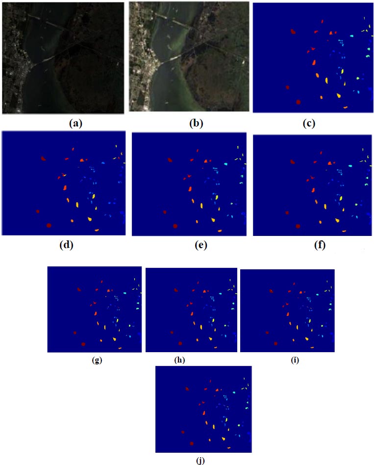
(c) 3DMWCNN [16] (d) GF_CNN [17] (e) DW-SDA [18] (f) MMS [19] (g) GFO [20] (h) PCA+SSA [21] (i) Proposed DBPNN (j) Proposed DRBFNN classifier.
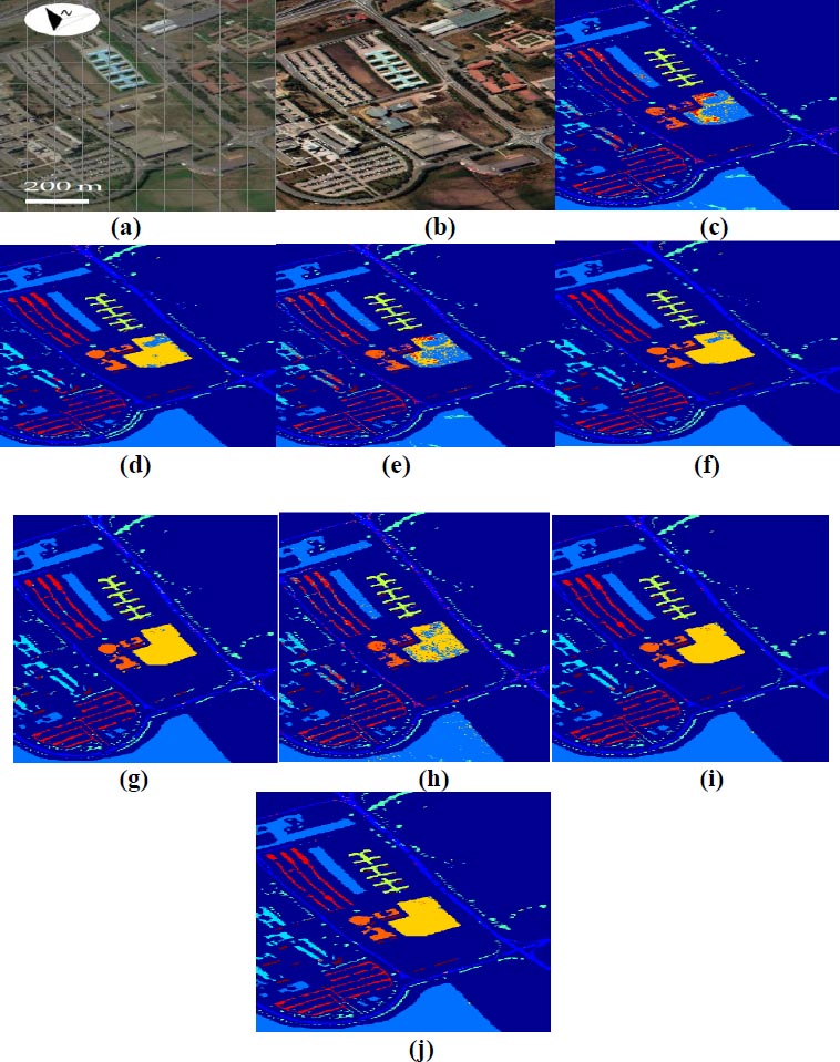
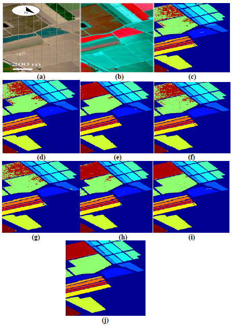
Fig. (8) showcases classified images for the University of Pavia datasets utilizing the proposed DBPNN and DRBFNN classifiers developed in this study. In Fig. (8a and b), the false color and RGB images are presented, respectively. The classification outcomes for University of Pavia datasets by 3 DMWCNN [16], GF+CNN [17], DW-SDA [18], MMS [19], GFO [20], PCA+SSA [21], DBPNN, and DRBFNN classifiers are displayed in Fig. (8c to j). DRBFNN, featuring Gaussian non-linear activation, achieves superior classification accuracy for the University of Pavia datasets, as evident in Fig. (8j). The image classification based on labeled classes with the new DRBFNN classifier surpasses other compared classifiers.
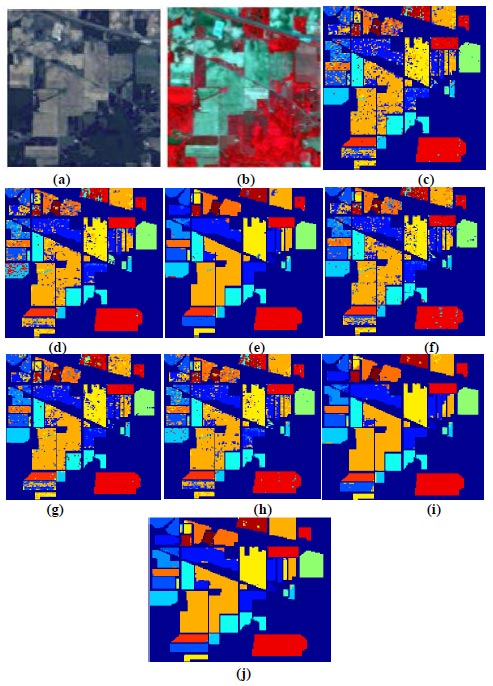
Fig. (9a,b) illustrates image classification results for Salinas datasets. A comparison of classified images by various classifiers (3DMWCNN [16], GF+CNN [17], DW-SDA [18], MMS [19], GFO [20], PCA+SSA [21], DBPNN, and DRBFNN) is presented from Fig. (9c to j). Notably, in Fig. (9j), the proposed DRBFNN classifier exhibits highly superior classification for Salinas datasets, attributed to the Gaussian non-linear activation function. Similarly, for Indian Pine datasets, Fig. (9j) distinctly showcases the superior performance of the new DRBFNN classifier compared to all other classifiers considered. The DRBFNN, with Gaussian activation function, achieves better accuracy (Acccl) and minimized error (Errormse) for numerous labelled classes in the Indian Pines dataset, surpassing other classifiers in the comparison set.
5. COMPARATIVE AND STATISTICAL ANALYSIS
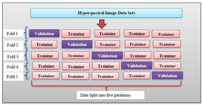
In training the newly developed deep learning classifier for hyperspectral image datasets (KSC, University of Pavia, Salinas, and Indian Pine), the data are partitioned into training (60%), testing (20%), and validation (20%) sets. Uniform data distribution is ensured across all sets through basic regression, defining class boundaries uniformly. The proposed deep learning classifiers undergo training, testing, and calibration for all considered datasets. 5-fold cross-validation is employed, dividing the 20% testing data equally into five parts for validation in each iteration (Fig. 10a-j). Fig. (11) illustrates the 5-fold cross-validation process. Accuracy is evaluated and tabulated for all datasets using the proposed models. To validate the superiority of the developed DBPNN and DRBFNN classifiers, comparisons are made with various classifier approaches, including
- 3D multi-resolution wavelet convolutional neural networks [16]
- Gabor filtering and convolutional neural network [17]
- Dual-Window Superpixel Data Augmentation [18]
- Modified-mean-shift-based noisy label detection [19]
- Gradient Feature-Oriented 3-D Domain Adaptation [20]
- PCA and segmented-PCA domain multi-scale 2-D-SSA [21]
| Average Classification Accuracy (%) | ||||
|---|---|---|---|---|
| Classifiers for Comparison from State-of-the-art Techniques/Refs. | KSC Datasets | Pavia University Datasets | Salinas Dataset | Indian Pine Datasets |
| 3DMWCNN classifier [16] | 96.22 | 95.91 | 97.17 | 94.28 |
| GF+CNN approach [17] | 97.60 | 96.95 | 98.06 | 82.54 |
| DW-SDA approach [18] | 95.42 | 93.69 | 97.04 | 97.23 |
| MMS technique [19] | 74.43 | 96.11 | 90.44 | 97.13 |
| GFO learning model [20] | 87.09 | 93.94 | 92.58 | 72.51 |
| PCA+SSA classifier [21] | 94.74 | 97.85 | 98.64 | 96.13 |
| Proposed DBPNN Classifier | 97.38 | 97.25 | 97.40 | 97.67 |
| Proposed DRBFNN Classifier | 97.91 | 98.04 | 98.69 | 98.27 |
Table 10 presents a comparison of mean classification accuracy across the four hyperspectral image datasets, evaluating the proposed DBPNN and DRBFNN classifiers against state-of-the-art models. For the KSC, Pavia, Salinas, and Indian Pine datasets, the average accuracy (Acccl) with DBPNN is 97.38%, 97.25%, 97.40%, and 97.67%, and with DRBFNN is 97.91%, 98.04%, 98.69%, and 98.27%, respectively. These results affirm the superior mean classification accuracy of the developed DRBFNN classifier, outperforming techniques and even surpassing the proposed DBPNN. Table 10 records average accuracy values for each dataset, emphasizing the significance of the activation function for improved classifier performance. The distinctive features of each hyperspectral image dataset align with specific deep learning models, ensuring better accuracy metrics with minimal error.
Table 11 details the elapsed training and testing times during MATLAB simulation for both deep learning classifiers across four hyperspectral image datasets. Comparative analysis reveals that 3DMWCNN, DLEM, and Deep ELM classifiers exhibit higher times than other approaches. Using the developed DBPNN classifier, the KSC dataset, Pavia, Salinas, and Indian Pine exhibit training times of 3.96s, 4.96s, 9.68s, and 6.22s, and testing times of 3.55s, 3.11s, 4.01s, and 3.24s, respectively. The modelled DRBFNN classifier shows shorter training times of 3.01s, 3.81s, 6.25s, and 5.03s and testing times of 2.86s, 2.79s, 3.49s, and 2.99s. Higher-end processors contribute to faster execution, reducing computational time during algorithm training and testing. Additionally, Table 11 outlines the elapsed training and testing epochs, indicating 21, 24, 29, 34, and 15, 13, 17, and 18 epochs for DBPNN across the four datasets. For DRBFNN, the epochs are 17, 21, 27, 29, and 12, 12, 17, and 16 for training and testing across KSC, University of Pavia, Salinas, and Indian Pine Datasets, respectively.
|
Hyperspectral Image Samples |
Existing and Proposed Classifiers for Comparison | Training Time (sec) | Testing Time (sec) | Training Epochs Elapsed | Testing Epochs Elapsed |
|---|---|---|---|---|---|
| KSC Datasets | 3DMWCNN classifier | 52.71 | 19.60 | 123 | 37 |
| GF+CNN approach | 26.78 | 11.76 | 93 | 29 | |
| Deep-ELM technique | 32.34 | 4.61 | 117 | 51 | |
| DD+SRM classifier | 30.98 | 12.30 | 63 | 32 | |
| DW-SDA approach | 48.17 | 8.70 | 44 | 26 | |
| DLEM classifier | 62.45 | 19.81 | 39 | 23 | |
| MMS technique | 13.62 | 12.22 | 52 | 25 | |
| FCSPN classifier | 9.81 | 9.45 | 37 | 19 | |
| GFO learning model | 4.22 | 3.82 | 25 | 16 | |
| Proposed DBPNN | 3.96 | 3.55 | 21 | 15 | |
| Proposed DRBFNN | 3.01 | 2.86 | 17 | 12 | |
| Pavia University Datasets | 3DMWCNN classifier | 36.71 | 21.45 | 109 | 38 |
| GF+CNN approach | 24.97 | 16.59 | 77 | 31 | |
| Deep-ELM technique | 18.20 | 15.56 | 147 | 43 | |
| DD+SRM classifier | 14.46 | 9.42 | 82 | 45 | |
| DW-SDA approach | 27.81 | 16.11 | 51 | 29 | |
| DLEM classifier | 32.29 | 21.13 | 47 | 23 | |
| MMS technique | 16.75 | 10.84 | 38 | 17 | |
| FCSPN classifier | 9.26 | 7.64 | 35 | 17 | |
| GFO learning model | 5.29 | 3.36 | 27 | 13 | |
| Proposed DBPNN | 4.96 | 3.11 | 24 | 13 | |
| Proposed DRBFNN | 3.81 | 2.79 | 21 | 12 | |
| Salinas Dataset | 3DMWCNN classifier | 56.92 | 18.47 | 136 | 57 |
| GF+CNN approach | 49.26 | 2.46 | 112 | 49 | |
| Deep-ELM technique | 27.81 | 10.27 | 127 | 53 | |
| DD+SRM classifier | 19.82 | 9.65 | 92 | 37 | |
| DW-SDA approach | 21.59 | 16.38 | 85 | 27 | |
| DLEM classifier | 30.42 | 20.36 | 61 | 38 | |
| MMS technique | 36.57 | 18.75 | 55 | 26 | |
| FCSPN classifier | 18.33 | 6.63 | 48 | 21 | |
| GFO learning model | 12.64 | 4.58 | 32 | 17 | |
| Proposed DBPNN | 9.68 | 4.01 | 29 | 17 | |
| Proposed DRBFNN | 6.25 | 3.49 | 27 | 17 | |
| Indian Pine Datasets | 3DMWCNN classifier | 67.92 | 18.54 | 105 | 51 |
| GF+CNN approach | 50.26 | 2.85 | 96 | 47 | |
| Deep-ELM technique | 36.57 | 14.52 | 65 | 34 | |
| DD+SRM classifier | 24.19 | 9.45 | 88 | 37 | |
| DW-SDA approach | 31.64 | 7.84 | 56 | 29 | |
| DLEM classifier | 27.84 | 6.98 | 72 | 31 | |
| MMS technique | 33.65 | 9.87 | 47 | 26 | |
| FCSPN classifier | 16.48 | 7.01 | 42 | 20 | |
| GFO learning model | 8.45 | 3.69 | 39 | 18 | |
| Proposed DBPNN | 6.22 | 3.24 | 34 | 18 | |
| Proposed DRBFNN | 5.03 | 2.99 | 29 | 16 |
Table 12 presents sensitivity and statistical analysis metrics for the new DBPNN and DRBFNN classifiers across all four HSI datasets. Sensitivity analysis, assessing the impact of input variables on dependent parameters, is conducted by observing changes in training mean square error upon removing inputs [22]. Delta error and average absolute gradient indicate ranking performance and input perturbation monitoring, respectively, and demonstrate minimal values for all datasets using the proposed DBPNN and DRBFNN classifiers. Statistical validation, employing correlation coefficient and determination measure, yields values close to 1 across the tested HSI datasets, affirming the validity of the proposed deep learning classifier algorithm.
The delta error, representing the disparity between target and output values for system input variables, gauges convergence, and model accuracy in the developed deep neural network. Minimal delta error ensures convergence, enhancing generalization and learning. Table 12 reveals delta errors of 0.0057, 0.0052, 0.0046, and 0.0029 for KSC, University of Pavia, Salinas, and Indian Pine datasets, respectively, with the deep radial basis function neural network classifier. These values, within the range of 10-3, affirm minimized error during deep training, confirming robust learning and generalization in the proposed classifiers. The average absolute gradient, derived during the application of gradient descent learning, reflects the error gradient's impact on classification accuracy. Table 12 reports values of 0.1761, 0.1096, 0.0913, and 0.0905 for KSC, University of Pavia, Salinas, and Indian Pine datasets, respectively, with the DRBFNN classifier. The minimal absolute gradient underscores the classifier's effectiveness, which is rooted in the error gradient within the weight update mechanism of the gradient descent learning rule.
|
Proposed Classifiers |
Datasets | Sensitivity Analysis | Statistical Analysis | |||
|---|---|---|---|---|---|---|
|
Spectral Band and Step Size |
Delta Error | Average Absolute Gradient | Correlation Coefficient | Determination Measure | ||
|
DBPNN Classifier |
KSC Datasets | [5, 50] with step 5 |
0.0065 | 0.1980 | 0.9896 | 0.9961 |
| University of Pavia dataset | [5, 50] with step 5 |
0.0059 | 0.1249 | 0.9937 | 0.9959 | |
| Salinas dataset | [10,100] with step 10 | 0.0061 | 0.1045 | 0.9979 | 0.9890 | |
| Indian Pine Datasets | [10,100] with step 10 | 0.0033 | 0.0992 | 0.9901 | 0.9927 | |
|
DRBFNN Classifier |
KSC Datasets | [5,50] with step 5 |
0.0057 | 0.1761 | 0.9915 | 0.9966 |
| University of Pavia dataset | [5, 50] with step 5 |
0.0052 | 0.1096 | 0.9927 | 0.9939 | |
| Salinas dataset | [10,100] with step 10 | 0.0046 | 0.0913 | 0.9936 | 0.9886 | |
| Indian Pine Datasets | [10,100] with step 10 | 0.0029 | 0.0905 | 0.9899 | 0.9903 | |
CONCLUSION
This case introduces innovative deep learning classifiers, including a back propagation neural network (DBPNN) and a radial basis function neural network (DRBFNN), for hyperspectral image classification. The DBPNN incorporates deep auto-encoders and decoders, featuring a nine-layer architecture, and undergoes training, testing, and validation using KSC, University of Pavia, Salinas, and Indian Pine datasets. The DRBFNN, with a seven-layer architecture and Gaussian activation function, demonstrates superior efficacy in classification accuracy and mean square error during training convergence. Both classifiers surpass previous models in accuracy and error minimization. Notably, the DRBFNN outperforms the DBPNN and other models. Statistical and sensitivity analyses reveal insights into input perturbations and classified outputs. Future research aims to extend this work by exploring novel deep recurrent neural network classifiers, aiming to simplify structural complexity and leverage memory states from previous layers. Limitations of this study include the potential limited generalizability of the proposed deep learning models, DBPNN and DRBFNN, beyond tested datasets, as well as uncertainty regarding optimal hyperparameter selection, computational resources, and evaluation metrics capturing the nuances of hyperspectral image classification. To address these limitations, further validation of diverse datasets, sensitivity analyses on hyperparameters, comprehensive computational resource analysis, and exploration of additional evaluation metrics are recommended.
LIST OF ABBREVIATIONS
| FFNN | = Feed-Forward Neural Networks |
| DBPNN | = Deep Backpropagation Neural Network Classifier |
| DRBFNN | = Deep Radial Basis Function Neural Network Classifier |
| ReLU | = Rectified Linear Unit |
| KSC | = Kennedy Space Centre |
| MSE | = Mean Square Error |