All published articles of this journal are available on ScienceDirect.

Feature Selection Techniques for the Analysis of Discriminative Features in Temporal and Frontal Lobe Epilepsy: A Comparative Study
Authors Info & Affiliations
Abstract
Background:
Because about 30% of epileptic patients suffer from refractory epilepsy, an efficient automatic seizure prediction tool is in great demand to improve their life quality.
Methods:
In this work, time-domain discriminating preictal and interictal features were efficiently extracted from the intracranial electroencephalogram of twelve patients, i.e., six with temporal and six with frontal lobe epilepsy. The performance of three types of feature selection methods was compared using Matthews’s correlation coefficient (MCC).
Results:
Kruskal Wallis, a non-parametric approach, was found to perform better than the other approaches due to a simple and less resource consuming strategy as well as maintaining the highest MCC score. The impact of dividing the electroencephalogram signals into various sub-bands was investigated as well. The highest performance of Kruskal Wallis may suggest considering the importance of univariate features like complexity and interquartile ratio (IQR), along with autoregressive (AR) model parameters and the maximum (MAX) cross-correlation to efficiently predict epileptic seizures.
Conclusion:
The proposed approach has the potential to be implemented on a low power device by considering a few simple time domain characteristics for a specific sub-band. It should be noted that, as there is not a great deal of literature on frontal lobe epilepsy, the results of this work can be considered promising.
1. INTRODUCTION
Epilepsy is the second most common and devastating neurologic disease, which affects over 70 million people around the world [1–5]. For some patients, it can be managed with antiepileptic medications or surgery. However, 20 to 30% of them would likely get worse after the initial diagnosis, and some may even become refractory to the current medicine [4, 5]. Anticipating seizures enough in advance could allow patients and/or caretakers to take appropriate actions and therefore, reduce the risk of injury [6].
Seizure is an irregular neural activity in the form of a sudden uncontrolled electrical discharge in the cortical brain regions. As a result, a collection of nerve cells start firing excessively and synchronously. People with frequent and unprovoked seizures are usually diagnosed as epileptics [7], [8].
Intracranial EEG (iEEG) is an electroencephalography recording utilizing intracranial electrodes implanted in the brain and require a surgical procedure [4]. So, compared to the scalp electrodes, EEG is less noisy and seizures can be identified typically earlier through the intracranial electrodes [6, 9].
The International League Against Epilepsy (ILAE) divided epileptic seizures into partial or focal and generalized seizures. Focal seizures originate in a limited region of the brain and may spread to other regions. On the other hand, generalized seizures are initiated in bilateral hemispheric areas and quickly propagate to all cortical areas [10]. Though there are different forms of seizures, we focused on those that are focal, mainly in the temporal and frontal lobes, entitled to Temporal Lobe Epilepsy (TLE) and Frontal Lobe Epilepsy (FLE), respectively.
TLE is one of the most prevalent forms of focal epilepsy. It has received a significant amount of attention from neurologists due to its high likelihood of clinical occurrence [11–14]. This kind of epilepsy may be treated medically at the onset of the disease with different antiepileptic drugs [14].
FLE is the second-most common form of focal epilepsy after TLE accounting for 25% of epilepsy [15–18]. Instead, FLEs, as compared to TLEs, tend to be brief, drug-resistant, more problematic, and to occur during sleep. Furthermore, the surgery for FLE has poorer outcomes than for TLE; as a result, the surgical workup of FLE is even more demanding [15, 19], [20]. Diagnosis of the FLE is rather hard due to having similar symptoms as a sleep disorder, or night terror, and psychiatric diseases [19]. Regarding the detection of FLE, some works have been published by analyzing various signals in the body such as EEG, ECG (Electrocardiography), EMG (Electromyography), and EOG (Electrooculography) [19], [21–25]. One report about the prediction of frontal lobe epilepsy on WAG/Rij rats was published [15] and to the best of the authors’ knowledge, no previous studies have been reported in the prediction of frontal lobe epilepsy of humans. Then, implementing a prediction system for FLEs is crucial due to the lack of supervision at night.
Several feature extraction techniques have been introduced in the last few years, among them, the time-domain ones are the earliest recommended methods. Time-domain features are employed to achieve discriminative information at a low computational cost. The obtained features are then fed to feature selection method [26]. High-quality features can be defined as those that produce maximum class separability, robustness, and less computational complexity. In this research, the general impact of iEEG signal variations on 16 commonly used features was investigated.
Designing and implementing a reliable forecasting and early warning tool that can help epileptic individuals to take appropriate drugs during an early warning period is, therefore, vital [27–29]; it will significantly improve their life quality. Furthermore, since portable devices are so available in daily life, targeting tools that can be easily implemented in such devices is the main objective of this study.
To this aim, the tool should enhance the daily life of the patients and increase their autonomy. However, knowing that:
- for new customers, the application will have to be frequently updated during its first uses to be able to integrate the new patient data efficiently,
- some patients may not have regular access to wireless connections and/or computers/tablets,
the opted strategy was to consider a dual-mode operation: the training/update should be performed on the portable device itself while the application is still working on prediction mode. So, in order to ensure an efficient online training/prediction, it is crucial to shorten the training CPU (Central Processing Unit) time while making the tool operation as simple as possible. This tool will then have to integrate such constraints.
One of the limitations of published works in this field is about employing few limited data in their studies. The authors attempted to study just one minute of data [30] or they used a limited amount of data: 5 min preictal and 10 min interictal [31]. Another notable limitation of existing works is filtering the EEG signal with a pass-band filter, which removes the high-frequency sub-bands that are very important in the prediction of the seizure [32, 33]. The plan is to use a wide range of frequencies (up to 120 Hz) and consider the whole available data for the nominated patients.
Several feature extraction techniques have been introduced in the last few years, among them the time-domain ones are the earliest recommended methods. Time-domain features are employed to achieve discriminative information at a low computational cost. The obtained features are then fed to feature selection methods [26]. High-quality features can be defined as those that produce maximum class separability, robustness, and less computational complexity, a key parameter to consider while targeting their use in portable devices. In this research, the general impact of iEEG signal variations on 16 commonly used features was investigated. However, little evidence has been reported on the effectiveness of various feature selection methods on EEG data of epilepsy patients. Therefore, it is required to explore their differences and find which one may work better than the others in perspective to deploy such algorithm in an implantable medical device that uses linear features, which allows rapid calculation with less complexity in prediction of the seizure.
2. MATERIALS AND METHODS
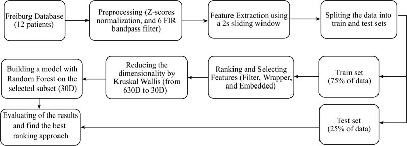
The proposed method steps are illustrated in Fig. (1). In the first phase, as detailed in the appendix, six EEG signals are preprocessed and 16 features extracted (these features being adopted from previous studies). Then, the data are divided into train and test sets and three kinds of feature selection methods employed to reduce the data dimension, making the approach computationally efficient. Next, the obtained results are tested by a well-known judging classifier namely, Random Forest. The 30 top extracted important features are ranked by various methods and fetched into the Random Forest classifier, while Mathew’s correlation coefficient (MCC) is used to analyse the performance. Finally, the relevant features among the 30 top ones are retained for the winner feature selection method.
2.1. EEG Database
The EEG dataset employed in this research is from the University Hospital of Freiburg, Germany. The EEG-database consists of two sets of files: “preictal (pre-seizure) data,” i.e. epileptic seizures with at least 50 min preictal data, and “interictal data,” which contains about 24 hours seizure-free EEG-recordings. The EEG-database comprises six iEEG electrodes from 21 patients with a sampling rate of 256 Hz. In this work, the participants are divided into two groups based on the origin of their seizures. In this study, 12 epilepsy patients (six TLE with the hippocampal and origins (134 hours) and six FLE with neocortical origin (137 hours)), i.e., the set of data available in the Freiburg database (Appendix B) were retained [34].
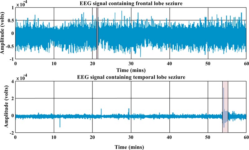
In Fig. (2), one-hour iEEG data (single channel) from a patient with frontal and an individual with temporal lobes is depicted. As one can see, epilepsy from the frontal lobe (which takes about 7 seconds) is shorter than the temporal one (which takes about 91 seconds). In addition, the morphology of the signal over a given period of time for each type of epilepsy is completely different. In fact, one can observe some hints in the preictal stage of the temporal one that is not in the other one.
2.2. Feature Extraction
The preliminary stage in EEG signal analysis is preprocessing. To decrease the effect of factors that cause baseline differences among the different recordings within the dataset and remove the signal DC component, iEEG signals were normalized using Z-score (expressed in terms of standard deviations from their means). The only potential artifact that could be addressed was the harmonic power line interference at 50 Hz. The 50 Hz interference was indirectly eliminated by performing the sub-band filtering which Gamma was divided into two sub-bands.
To deal with imbalanced dataset, an hour EEG signal was divided into 2 seconds non-overlapping windows for the interictal section, while the preictal section was split into chunks of the same window sizes with 50% overlapping. Various univariate linear measures were extracted at each epoch of two seconds along with a bivariate linear measure, as reported in Table 1. [35–39]. These time domain features, well-known in seizure forecasting, are explained in detail in Appendix A.
| S. NO. | Features | Comments | Time of the Computation for Each Channel (s) |
|---|---|---|---|
| 1 | Energy | One feature (36D)1 | 0.001593 |
| 2 | Mean | One feature (36D) | 0.018089 |
| 3 | Variance (VAR) | One feature (36D) | 0.011741 |
| 4 | Skewness | One feature (36D) | 0.181114 |
| 5 | Kurtosis | One feature (36D) | 0.014463 |
| 6 | Interquartile range (IQR) | One feature (36D) | 0.036152 |
| 7 | Zero Crossing Rate (ZCR) | One feature (36D) | 0.007410 |
| 8 | Mean Absolute Deviation (MAD) | One feature (36D) | 0.010459 |
| 9 | Entropy | One feature (36D) | 1.168083 |
| 10 | Hjorth mobility | One feature (36D) | 0.007360 |
| 11 | Hjorth complexity | One feature (36D) | 0.003935 |
| 12 | Coefficient of Variation (CoV) | One feature (36D) | 0.010528 |
| 13 | Root Mean Square (RMS) | One feature (36D) | 0.171703 |
| 14 | MAX2 cross correlation | 15 values for 6 channels, but one feature was considered (90D) | 0.087968 (between two channels) |
| 15 | AR3 model | Two features 4 (72 D) | 0.026372 |
Prior to feature extraction, six band-pass FIR (Finite Impulse Response) filters were utilized to divide the iEEG signals into different frequency bands: Delta (0.5-4 Hz), Theta (4-8 Hz), Alpha (8-12 Hz), Beta (12-30 Hz), as well as two Gamma bands namely, low-Gamma (30-47 Hz), and high-Gamma (53-120 Hz) [40–42]. This led to an input space of 630 features (dimensions) for each window.
2.3. Feature Selection
Feature selection is a vital stage in analyzing the data to improve model performance and reduce mathematical computational complexity by projecting the existing features onto a lower dimensional space. This technique reduces the input dimensionality by removing irrelevant or redundant features from the entire feature set [32, 43–47]. In the machine learning literature, the approaches to feature subset selection are often categorized as filter, wrapper, and embedded strategies [44, 46–48].
Filter approaches are based on the statistical properties of explanatory variables (predictor variables) and their relationship to the outcome variable (response); they are basically not computationally expensive. There are a lot of filter methods such as PCA (Principal Component Analysis), LDA (Linear Discriminant Analysis), and PLS (Partial Least Squares) which all find the linear combination of features to characterize two or more classes. However, even if they are linear, simple, and relatively low cost to reduce the dimensionality of the data, there is no clear interpretation of the feature ranking. Moreover, PCA as a famous feature reduction method is an unsupervised method, which does not consider dependent variables [49–51].
We employed the Kruskal Wallis (KW), a nonparametric test, without making prior assumptions about the data distribution, unlike the One Way ANOVA [52], [53].
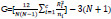
The value of Kruskal-Wallis ranking can be calculated as the following equation:
 |
(1) |
N is the total number of observations across all classes, ni is defined as the number of observations in group i, Rj is the mean rank of group i, c is the number of output group [53].
Wrapper approaches try to find a predictive model by using various combinations of features, then select the set of features that offer the highest evaluation performance. These techniques can be time consuming and tend to be slow. Therefore, they are not appropriate for large-scale problems to select the subset of features. One of the most popular wrapper techniques, Support Vector Machine- Recursive Feature Elimination (SVM-RFE), was used which backward eliminate features [54], [55]. The backward elimination technique builds a model on the entire set of all features and computes an importance score for each one. Then it removes the least significant features at each iteration which enhances the performance of the model. In other words, the top ranked variables are eliminated last [54–56].
Embedded techniques are inbuilt feature selection, allowing a classifier to build a model that automatically performs attribute selection as a part of model training (performs feature selection and model fitting simultaneously) [44, 57]. In this work, XGBoost (Extreme Gradient Boosting) is used which has been broadly employed in many areas due to its parallel processing, high scalability and flexibility [58–63]. This embedded technique is optimized implantation of Gradient Boosting framework. Boosting is building a strong learner with higher precision with a combination of weaker classifiers and it is known as the Gradient Boosting once the weak classifiers in each phase are built based on the gradient descent to optimize the loss function [59–63]. To further improve it, the XGBoost classifier has two regularization terms (inbuilt L1 and L2) to penalize the complexity of the model and avoid overfitting [59, 60, 63].
2.4. Evaluation and Performance Analysis
After extracting a number of features to discriminate between the preictal and interictal periods, 30 attributes that held the most discriminative information were deemed. We extracted from three approaches and then applied each new group of features to one of the most powerful ensemble methods, Random Forest. This embedded approach belongs to bagging for judging the performance of the other attribute selectors and it differs from boosting mechanism [64–66]. It should be noted that a bagging classifier is selected rather than boosting one to avoid systematic bias in the comparison results.
A classifier must be generalized, i.e., it should perform well when submitted to data outside the training set. Owing to the issue of class imbalance, accuracy could be an inadequate metric to evaluate the performance of the classifier [67–70]. Although accuracy remains the most intuitive performance measure, it is simply a ratio of correctly predicted observations over the total observations, so reliable only when a dataset is symmetrical. However, this measure has been used exclusively by some researchers in analyzing seizures [71–73].
Numerous metrics have been developed to analyze the effectiveness and efficiency of the model in handling the imbalanced datasets, such as F1 score, Cohen’s kappa, and MCC [68–70]. Among the above popular metrics, MCC is revealed as a robust and reliable evaluation metric in the binary classification tasks and, in addition, it was claimed that measures like F1 score and Cohen’s kappa should be avoided due to the over-optimism results especially on unbalanced data [68, 69, 74, 75].
To visualize and evaluate the performance of a classifier, the confusion matrix was used (see Table (2), which represents the confusion matrix of a binary classification). After computation of the confusion matrices, it should be noted that MCC has been retained to compare the classification performance and effectiveness of the feature selection methods.
| Actual | Predicted | |
|---|---|---|
| Positive | Negative | |
| Positive | TP (True Positive) | FN (False Negative) |
| Negative | FP (False Positive) | TN (True Negative) |
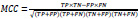
2.3.1. Matthews’s Correlation Coefficient (MCC)
MCC takes into account all four quadrants of the confusion matrix, which gives a better summary of the performance of classification algorithms. MCC can be considered as a discretization of the Pearson’s correlation coefficient for two random variables due to taking a possible value in the interval between -1 and 1 [75–77]. The score of 1 is deemed to be a complete agreement, −1 a perfect misclassification, and 0 indicates that the prediction is no better than random guessing (or the expected value is based on the flipping of a fair coin).
 |
(2) |
3. RESULTS
3.1. Dividing Signals Into Frequency Sub-bands
The aim of this study is to analyze and rank the time-domain features introduced by other researchers related to epileptic seizures in forecasting with EEG signals and compare the performance of three feature selection approaches based on the interictal and pre-ictal segments. Given the goal of classifying iEEG data into two classes: “1” denoting the ictal stage and the period preceding a seizure and “0” denoting seizure-free periods (interictal) and postictal (the time following a seizure).
Before ranking the features and comparing them, one needs to investigate how much dividing EEG signal into various sub-bands can be important. Therefore, a comparison of the accumulated energy for two cases, without and with dividing the signal into 6 sub-bands, was performed. The feature selection scores have represented both lobes in Fig. (3). The result for both graphs shows that dividing the EEG signal into various sub-bands can improve the performance of seizure forecasting because it contains much more discriminative information than the other case. Interestingly, the dimensionality of data will be increased for now but, later, the focus will be on specific sub-bands and reducing the dimensional feature space to consume less memory at runtime.

3.2. Feature Selection Methods Comparison
It should be noted that three methods for feature ranking were employed and afterwards independent train and test sets were defined to compare their performance using a Random Forest classifier. To have a better estimation of the generalization performance of the work, we evaluated the top 30 selected attributes on the testing dataset, which has not been used during the training process.
Using MATLAB, the calculations are made on an Intel(R) Core (TM) i7CPU 3.3GHz, and 16 GB RAM. Once the preprocessing stage was covered in MATLAB, MAT files were converted to NumPy arrays and the rest of the work in Python (3.7.6) programming language was developed. The computation time for each feature selection method is listed in Table (3) and the performance of the various feature selection methods is listed in Table (4).
| Brain lobe/Selection method | Kruskal-Wallis | SVM-RFE | XGBOOST |
|---|---|---|---|
| Temporal lobe | 12.4 min | 3411 min | 18.7 min |
| Frontal lobe | 10.9 min | 2375 min | 12 min |
By comparing the two above tables, it can be concluded that the filter-based method, Kruskal Wallis, has the highest MMC score and less computation time, while SVM-RFE has a longer computation time compared to the other approaches and shows the poorest performance.
It is worth mentioning that, in several existing publishing works, the researchers commonly selected nearly 5% of the feature sets and investigated the related sensitivity. In this work, 10, 20, and 50 dimension cases were examined and a compression made with 30D based on the MCC score in Table (5), highlighting the KW approach as the winner. The results of both lobes obviously demonstrate an increase in MCC score while is computationally expensive and time consuming.
| Selection method | MCC score | |
|---|---|---|
| performance | Temporal lobe | Frontal lobe |
| Kruskal-Wallis | 0.55±0.003 | 0.24±0.003 |
| SVM-RFE | 0.40±0.003 | 0.11±0.002 |
| XGBOOST | 0.496±0.003 | 0.12±0.002 |
Table 5.
| The number of dimensions | MCC score | |
|---|---|---|
| Temporal lobe | Frontal lobe | |
| 10D | 0.44 | 0.07 |
| 20D | 0.50 | 0.12 |
| 30D | 0.55 | 0.24 |
| 50D | 0.57 | 0.26 |
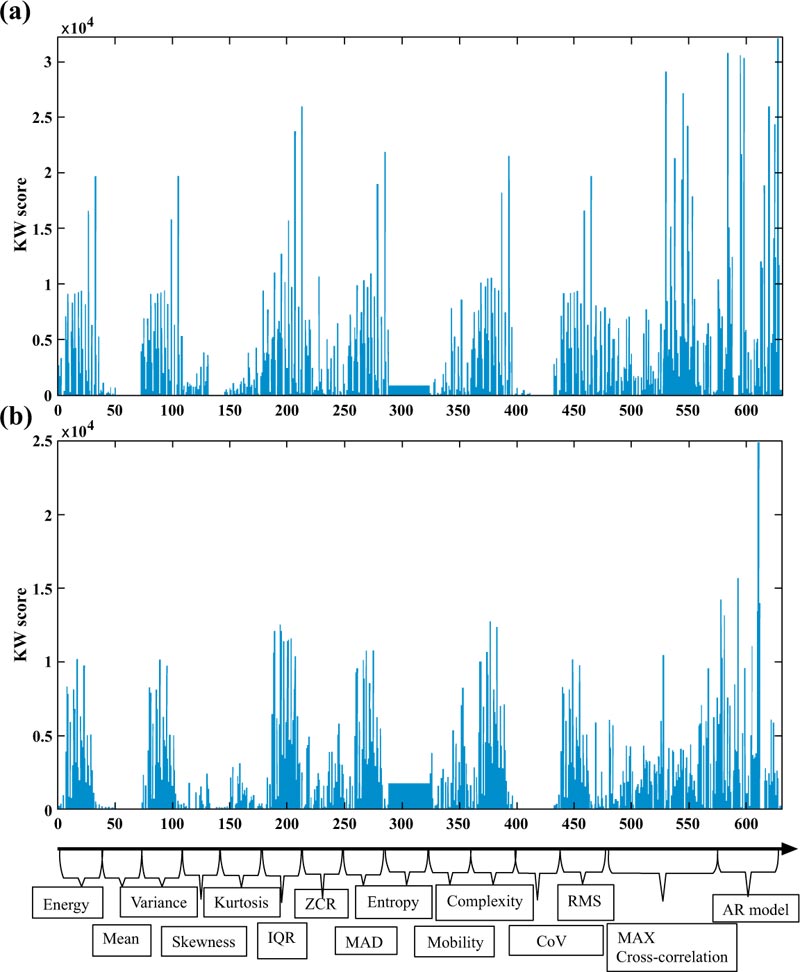
The top 30 ranked subsets are listed in Tables (6 and 7) for TLE and FLE, respectively, based on the three feature selection approaches. The most popular feature ranked by the three feature selection methods is AR. The second most important feature is the MAX cross-correlation and complexity is the next one. Interestingly, features like Mean, Skewness, Zero Crossing Rate, and Entropy are not deemed as top 30 ranked feature-subset as in Tables (6 and 7). Also, the following remarks can be made:
| Top Features | KW | SVM-RFE | XGBOOST |
|---|---|---|---|
| 1 | AR High-Gamma error | MAX cross Beta | AR error Beta |
| 2 | AR Alpha error | AR Delta coefficient | AR Beta error |
| 3 | AR Beta coefficient | MAX cross High-Gamma | AR High-Gamma error |
| 4 | AR Beta error | MAX cross Beta | AR Low-Gamma error |
| 5 | MAX cross Low-Gamma | MAX cross Beta | AR Theta Error |
| 6 | MAX cross High-Gamma | MAX cross High-Gamma | AR Delta error |
| 7 | AR High-Gamma Error | RMS High-Gamma | AR Delta error |
| 8 | IQR High-Gamma | AR Theta coefficient | AR Alpha coefficient |
| 9 | AR High-Gamma coefficient | AR Theta Error | Complexity High-Gamma |
| 10 | MAX cross High-Gamma | RMS Beta | AR Delta coefficient |
| 11 | IQR High-Gamma | AR Beta coefficient | AR High-Gamma error |
| 12 | MAD High-Gamma | MAX cross Beta | AR Delta error |
| 13 | AR Beta error | MAX cross Delta | Complexity Beta |
| 14 | Complexity High-Gamma | MAX cross Delta | AR Alpha coefficient |
| 15 | MAX cross Low-Gamma | CoV Low-Gamma | MAD High-Gamma |
| 16 | VAR High-Gamma | MAX cross Alpha | AR Alpha error |
| 17 | Energy High-Gamma | RMS Delta | MAX cross High-Gamma |
| 18 | RMS High-Gamma | MAX cross Low-Gamma | AR High-Gamma error |
| 19 | MAX cross High-Gamma | RMS Theta | AR coefficient Alpha |
| 20 | MAD High-Gamma | MAX cross Beta | AR High-Gamma coefficient |
| 21 | AR Low-Gamma error | RMS Delta | AR Beta coefficient |
| 22 | Complexity Low-Gamma | RMS Low-Gamma | AR Beta coefficient |
| 23 | MAX cross High-Gamma | Complexity High-Gamma | AR Beta error |
| 24 | VAR Low-Gamma | Mobility Delta | AR Alpha coefficient |
| 25 | Energy Low-Gamma | Mobility Low-Gamma | IQR Beta |
| 26 | RMS Low-Gamma | MAX cross Delta | AR Delta coefficient |
| 27 | IQR Low-Gamma | Complexity Alpha | AR Delta error |
| 28 | MAX cross Low-Gamma | Complexity High-Gamma | AR Alpha error |
| 29 | AR coefficient Alpha | Complexity Low-Gamma | AR Low-Gamma coefficient |
| 30 | AR High-Gamma error | Complexity Delta | Mobility Delta |
| Top Features | KW | SVM-RFE | XGBOOST |
|---|---|---|---|
| 1 | AR Low-Gamma error | AR High-Gamma error | AR delta coefficient |
| 2 | AR Alpha coefficient | AR Alpha error | AR Theta error |
| 3 | AR Theta error | MAX cross High-Gamma | AR Delta coefficient |
| 4 | AR Low-Gamma error | AR Theta coefficient | AR Theta error |
| 5 | AR Low-Gamma error | MAX cross Beta | AR Theta error |
| 6 | AR Theta error | AR Delta error | AR Delta error |
| 7 | Complexity Alpha | MAX cross Alpha | AR Low-Gamma error |
| 8 | IQR Alpha | MAX cross Beta | AR Alpha coefficient |
| 9 | Mobility Beta | AR Delta error | AR Alpha error |
| 10 | IQR Alpha | RMS Low-Gamma | AR Alpha error |
| 11 | IQR Theta | MAX cross Delta | AR Theta coefficient |
| 12 | IQR Beta | RMS High-Gamma | AR Beta coefficient |
| 13 | IQR Low-Gamma | MAX cross Alpha | AR Beta error |
| 14 | IQR Alpha | Complexity Alpha | Kurtosis High-Gamma |
| 15 | Kurtosis Beta | MAX cross High-Gamma | AR Beta error |
| 16 | AR Beta coefficient | MAX cross Beta | AR Low-Gamma coefficient |
| 17 | MAD Alpha | MAX cross Theta | AR Beta coefficient |
| 18 | MAD Beta | MAX cross Low-Gamma | AR High-Gamma error |
| 19 | Complexity Alpha | MAX cross Beta | AR Beta coefficient |
| 20 | IQR Theta | RMS Delta | AR Beta error |
| 21 | AR Beta Error | MAX cross Alpha | AR High-Gamma error |
| 22 | IQR High-Gamma | MAX cross Theta | AR Delta coefficient |
| 23 | AR Theta coefficient | Complexity Delta | AR High-Gamma error |
| 24 | Energy Alpha | RMS Low-Gamma coefficient | AR Delta error |
| 25 | RMS Theta | Mobility Alpha | AR High-Gamma coefficient |
| 26 | VAR Alpha | Complexity High-Gamma | AR Delta error |
| 27 | MAD Alpha | Mobility Alpha | AR High-Gamma error |
| 28 | Complexity Theta | Complexity Low-Gamma | AR Theta coefficient |
| 29 | Complexity Theta | Complexity Delta | MAD Beta |
| 30 | Energy Beta | Mobility High-Gamma | AR Delta coefficient |
- AR model is an interesting feature along with MAX cross correlation for all three feature selection methods and both lobes
- Delta sub band is considered an important sub band for XGBOOST and SVM-RFE, but not the case for Kruskal Wallis
- Error is more important than coefficient as AR parameters in discriminating feature between seizure and non-seizure for all three feature selection methods
Some of the attributes were selected multiple times by the feature ranking approaches in both Tables, like AR High-Gamma Error which has been chosen by Kruskal Wallis as feature 1, 7, and 30 in Table (6). The reason behind that is such features have been selected and presented without considering the order of the electrodes.
Figs. (4a and 4b) illustrate an overview of the features selected with the KW for temporal and frontal lobes, respectively. Fig. (4a) confirms that amongst the Time-domain parameters that play an important role in the prediction of the seizure, AR is the top feature, followed by the cross correlation and the IQR. On the other hand, Fig. (4b) shows that the AR model, a measure of complexity obtained with Hjorth’s analysis, is an important feature besides IQR for patients with frontal lope epilepsy.
In the last step, another filtering method is applied to obtain the product-moment correlation coefficient, or Pearson correlation coefficient, in order to identify the linear relationship between the 30 top ranked features and, therefore, to eliminate any redundant information. This coefficient can be expressed as
 |
(3) |
where Cov(X1, X2) is the covariance of two features and
| Lobes | Attributes with a Strong Linear Relationship |
|---|---|
| Temporal lobe | AR High-Gamma error / AR High-Gamma coefficient |
| IQR High-Gamma / MAD High-Gamma | |
| Energy High-Gamma / VAR High-Gamma | |
| Complexity High-Gamma / Complexity Low-Gamma | |
| VAR Low-Gamma / Energy Low-Gamma | |
| Frontal lobe | Complexity Alpha / Mobility Beta / Energy Beta |
| MAD Alpha / IQR Alpha / RMS Theta | |
| IQR Beta / MAD Beta | |
| Energy Alpha / VAR Alpha |
The product-moment correlation matrix was then calculated for the top 30 subset of features with the highest Kruskal-Wallis scores. The features with the strongest linear pattern are reported in Table (8). Interestingly, one can see a good relationship between IQR and MAD in both lobes, which has a strong linear relationship and it happens in Alpha and Beta sub-bands in frontal lobe and in low and high- Gamma sub-bands for temporal lobe. Also, there is a close relationship between variance and energy for both lobes.
4. DISCUSSION
For various reasons, some researchers have divided the EEG signal into various sub-bands [81, 82] while others have not [30, 39]. The aim was, therefore, to consider both cases and evaluate the impact of dividing the EEG signal into various sub-bands. In fact, as shown in Fig. (3), dividing the EEG signal into 6 sub-bands will carry more predictive information than not splitting it.
In this study, three feature selection methods were compared and the results showed that the filter method has the highest performance with the highest MCC. Also, KW can rank the features a lot faster, with the shortest computational time.
A large panel of wrapper approaches has been proposed for features selection but most of them are computationally expensive and complex in nature [53–55]. The results obtained in the study confirmed this fact: SVM-RFE has the lowest prediction performance and is the most intensive in terms of computation. Although, in most of the existing works, it has been claimed that the embedded methods that combine filters and wrappers take advantage of both, the obtained results did not really demonstrate that claim, showing that the non-parametric filter-based method, Kruskal Wallis, outperforms better than the above approaches.
The AR method estimates the power spectrum density (PSD) of a given signal. Then, this approach does not have the problem of spectral leakage and one can expect a better frequency resolution dissimilar to the nonparametric method. PSD can be estimated by calculating the coefficients even when the order is low [39, 83, 84]. Furthermore, the prediction error term extracted from an AR model of the brain signals is claimed to reduce during the preictal stage [85].
The maximum of cross-correlation, a bivariate feature, can be considered as a measure for lag synchronization due to estimating the phase difference between two spatially separated sensors even with a low SNR (Signal to Noise Ratio) [86], [87]. The key points for Kruskal Wallis as a winner can be due to not just considering the parameters of AR model and MAX cross coloration. This feature selection tried to engage other important univariate features like complexity, which has an estimation of statistical moment of the power spectrum.
The temporal lobe is responsible to deal with the processing of information and it plays a vital role in long term memory. Gamma rhythms are involved in higher processing tasks and cognitive functioning. These waves are the fundamental waves for learning, memory and information processing. The Frontal lobe is responsible for emotion control center, planning, judgment, and short-term memory. Theta rhythms are produced to help one in creativity, relaxation, and emotional connection. Alpha waves help in the feeling of deep relaxation and Beta waves are related to someone’s consciousness and problem solving [88].
In this study, it was found out that the low and high-gamma sub-bands are the most discriminating ones between preictal and interictal for TLE patients, while the frequency ranges from Theta to low-Gamma were found to be the most discriminating features in six patients with FLE. The obtained results confirmed that gamma sub-bands are a promising biomarker in predicting of seizure for TLE [89–91]. However, for FLE, one should consider a wider range of frequencies, including the lower frequency compared to TLE, in the preictal stage. Note that some existing works in detection of FLEs proposed that a range of frequencies less than 50 Hz can play dominant roles among different brain waves [22], [23], [92].
The results also demonstrated the complexity of seizure prediction due to the fact that the frontal lobes of the brain control a wide variety of complex structural and functional roles [15]– [17], [93]. These findings can help establish specific relationships regarding the impact of each lobe in a specific function and the generation of waveforms based on that function.
Furthermore, by comparing the performance results of Kruskal Wallis for both lobes in Table (4), MCC is not close to 1, the perfect prediction case. The reason for not having a high MCC is related to the low capacity of this version of Freiburg database due to having data up to 90 minutes of preictal, or to the fact that some seizures take few minutes. Based on Ramachandran et al. [71], it might be required at least 3 to 16 hours before the onset of the seizure to efficiently predict seizures which can be considered as a limitation in this study and weakness of this database. Another possible solution is employing non-linear measures, such as phase synchronization to improve the model performance in forecasting seizures.
Moreover, a non-stationary signal like EEG can be considered as a stationary signal in a short duration epoch, like a two-second window [94] and [95]. Also, based on the results in Figs. (4a and 4b), the variation of the mean feature for both lobes is nearly a constant value. This result partially confirms the previous claim, but this would require further investigations.
The effectiveness of the Kruskal Wallis as a nonparametric method is based on the fact that it does not need to assume a data distribution model, making the results promising in feature selection of EEG data of TLE and FLE. Therefore, dealing with a higher number of epilepsy patients will not be an issue and this approach would be applicable to a larger set of data. Furthermore, the data divided into train and test sets and the model was built by random forest was trained and validated with 10 fold cross validation. Also, we prevented overfitting, which can be considered as a generalized model for unseen data.
Furthermore, applying MCC in measuring the performance of the model, is a significant improvement over other existing works that deemed accuracy as the performance of the classifier while dealing with imbalanced data [31, 96–98]. Specifically, authors in [71] proposed an effective feature extraction method in improving classification accuracy while the imbalanced ratio was not reported and this performance metric was the only measure of the performance of the classifier.
It is believed that the findings of this work can be implemented on low power hardware by efficiently considering less complex features for a specific sub band with the information from only one patient, instead of building and deploying a model for the entire patients in the database.
CONCLUSION
The epileptic seizures are the temporary occurrence of symptoms due to synchronization of abnormally excessive activities of the brain nerve cells. However, reviewing the EEG signals will be a time consuming task for neurologists to analyze and monitor continuous electroencephalograms. Therefore, even it is quite challenging, implementing a high performance automated analysis of EEG signals is in high demand.
The Kruskal-Wallis feature selection strategy is simple and less time consuming as compared to other approaches. Among the time-domain features investigated, the parameters of AR model are ranked as the top features for both lobes. The second most important features are the maximum of cross-correlation and IQR for temporal and frontal lobes, respectively. Moreover, a high range of frequency like low and high-Gamma have been introduced as an interesting sub-band for the temporal lobe epilepsy, while the middle range of frequencies from Theta to Beta can be seen as important ranges of frequency for frontal lobe epilepsy.
Future efforts should be focused to reliably improve the performance of the prediction on test set for a patient-specific by considering a combination of various features which provide an estimation of phase, frequency and amplitude of the EEG signal.
AUTHORS CONTRIBUTIONS
software, B.A.; visualization, B.A.; writing—original draft preparation, B.A.; writing—review and editing, B.A., C.T., and M.C.E.Y.; supervision, C.T. and M.C.E.Y. All authors have read and agreed to the published version of the manuscript.
ETHICS APPROVAL AND CONSENT TO PARTICIPATE
Not applicable.
HUMAN AND ANIMAL RIGHTS
Not applicable.
CONSENT FOR PUBLICATION
Not applicable.
AVAILABILITY OF DATA AND MATERIALS
We used following database; we did not directly perform the tests ourselves:
https://pubmed.ncbi.nlm.nih.gov/17201704/
Predicting Epileptic Seizures in Advance (plos.org)
FUNDING
None.
CONFLICTS OF INTEREST
The authors declare no conflict of interest, financial or otherwise.
ACKNOWLEDGEMENTS
Declared none.
Appendix A
Feature is a variable that can represent the signal variation and in this work, common features were selected in analyzing EEG signal which discriminates between pre-ictal and interictal phases of the seizures.
Within a 2 s window, an EEG signal is first passed through six FIR band-pass filters, leading to a total of a 36-dimensional (36D) feature vector. Note that the dimensionality of MAX cross correlation among the 6 channels for each sub-band will be 90D. Then, extracting two features from the AR model (for each sub-band) will add a 72-dimension to the feature matrix, making a final a matrix of 630-dimensions.
In this study, 13 types of univariate features, a bivariate feature along two features extracted from AR model were investigated.
1. Energy:
This feature can be considered as a measure of the signal strength. Calculating the accumulated energy at a given time-point t, is a commonly used feature in finding abnormal behavior in the brain. For a given discrete signal, x(n), the area under the squared of a signal is called energy and is expressed as [36], [39]:
 |
2. Mean:
The mean of a discrete signal, x(n), can be expressed as [37]:
 |
Where N is the number of the samples and x(n) the discrete signal
3. Variance:
The second moment of a signal is called the variance. Higher its value, higher the number of frequency components the signal contains [87]
 |
4. Skewness:
The third statistical moment measures the asymmetry of the probability distribution about its mean.
 |
5. Kurtosis:
The fourth statistical moment describes the flatness of a distribution real valued random variable.
 |
6. Interquartile range:
The Interquartile Range (IQR) feature is a measure of spread and variability based on dividing the data into four equal parts. The separated values Q1, Q2, and Q3 for each part are named respectively first, second, and third quartiles. IQR is computed as the difference between the 75th and the 25th percentile or Q3 and Q1 as the following [38], [39]:
 |
7. Zero crossing rate:
The Zero Crossing Rate (ZCR) is the rate at which the signal changes signs or is the sum of all positive zero crossings into the EEG segment
8. Mean Absolute Deviation:
The robustness of the collected quantitative data can be calculated by MAD (Mean Absolute Deviation). In other words, it is the average distance between each data point and the mean. For a given dataset, x = x1, x2, … xn, MAD can be calculated as [38]:
 |
9. Entropy:
This feature is employed to quantify the degree of uncertainty and irregularity of a signal as well as the complexity of human brain dynamics. The uncertainty of the signal can be computed in terms of the repeatability of its amplitude [38]:
 |
Where P(x) is the probability mass function
10. Hjorth mobility:
The Hjorth mobility parameter represents the square root of the variance of the first derivative of the signal, and it is proportional to the standard deviation of the power spectrum of a time series.
 |
In the above equation, x(t) is a signal and x’(t) its derivative. var(-) is the variance of a signal over a period of time.
11. Hjorth complexity:
The Hjorth complexity defines how the shape of a signal is analogous to an ideal sine curve. This parameter gives an estimation of the bandwidth of the signal.
Complexity = mobility (x'(t)) / mobility (x(t))
One can have an estimation of the second and fourth statistical moment of the power spectrum in the frequency domain by employing the mobility and complexity, correspondingly. While Hjorth parameters are identified in time-domain, they can be useful for both time and frequency analysis. Interestingly, computation of the Hjorth parameters stands on variance, then the cost of their computation is significantly low [87, 99, 100].
12. Coefficient of Variation:
The coefficient of variation (CoV) is a measure is the division of the standard deviation to the mean of a signal [99]:
 |
13. Root Mean Square:
The Root Mean Square (RMS) of a signal can be calculated as [30]:
 |
14. Maximum linear cross-correlation:
As a simple bivariate measure, MAX cross-correlation calculates the linear association between two signals, which also yields fixed delays between two spatially distant EEG signals to accommodate potential signal propagation. This measure can also give us a similarity between two different channels.
Given an EEG signal containing N channels, one can compute the cross-correlation on
 pairs of channels (e.g. 15 pairs for N=6 for the employed iEEG database). Calculating the MAX cross correlation for six channels results in a 90-D vector.
15. Autoregressive (AR) model:
A sequence of observations ordered in time or space is called time-series and, in the electrical engineering context, is titled as signal. An AR model can be described by modeling the existing value of the variable as a weighted sum of its own preceding values. Similarly, one can employ this concept to forecast the future based on past behavior [101–103].
An AR model with order p can be described as the following formula:
 |
where εt is the error term, usually specified as white noise and β= (β1, β2,…, βp) is the AR coefficients.
For a first order, an AR(1) model can be expressed as [102–104]:
 |
and its process can be considered as a stationary process once |β1|<1. The coefficient and the error term have been considered as features in the prediction of the seizure [35, 87, 105].
Appendix B
The Freiburg EEG Database is one of the most cited resources employed in predicting and detecting experiments. The interictal and preictal intracranial electroencephalogram (iEEG) recordings of the Freiburg database (FSPEEG) was offered in the early 2000s as an EEG database [34]. The database consists of intracerebral (strips, grid and depth electrodes) EEG recordings from 21 epileptic patients. It contains six intracranial electroencephalography (iEEG) electrodes with a sampling frequency of 256 Hz and a 16-bit A/D converter.
The database contains 24 hours of continuous and discontinuous interictal recordings for 13 patients and eight patients, respectively. Each participant had 2 to 5 preictal recordings with about 50 minutes’ preictal recordings. This database contained 582 hours of EEG data, including preictal recordings of 88 seizures.
An overview of recruited patients is inserted in Table (9). Note that 50 seizures have been employed from 12 patients in this study (mean age: 31; age range: 14-50; both gender).
| Patient# | Sex | Age | Seizure type | H/NC | Origin | Electrodes | Seizures analyzed |
|---|---|---|---|---|---|---|---|
| 1 | F | 15 | SP, CP | NC | Frontal | g, s | 4 |
| 2 | M | 38 | SP, CP, GTC | H | Temporal | d | 3 |
| 3 | M | 14 | SP, CP | NC | Frontal | g, s | 5 |
| 4 | F | 26 | SP, CP, GTC | H | Temporal | d, g, s | 5 |
| 5 | F | 16 | SP, CP, GTC | NC | Frontal | g, s | 5 |
| 7 | F | 42 | SP, CP, GTC | H | Temporal | d | 3 |
| 8 | F | 32 | SP, CP | NC | Frontal | g, s | 2 |
| 10 | M | 47 | SP, CP, GTC | H | Temporal | d | 5 |
| 12 | F | 42 | SP, CP, GTC | H | Temporal | d, g, s | 4 |
| 16 | F | 50 | SP,CP, GTC | H | Temporal | d, s | 5 |
| 18 | F | 25 | SP, CP | NC | Frontal | s | 5 |
| 19 | F | 28 | SP, CP, GTC | NC | Frontal | s | 4 |