All published articles of this journal are available on ScienceDirect.
An Analysis of Electrocardiograms for Instantaneous Sleep Potential Determination
Abstract
Background:
The use of electrocardiograms to establish a relationship between the electrical activity of the heart and the intricacies of sleep is explored to propose a method to predict the time before sleep onset.
Recorded Electrocardiograms (ECG) from the National Sleep Research Resource (NSRR) database are analyzed to extract the frequency domain characteristics and used to develop statistical learning models to predict the time before sleep onset. This is known as Time to Sleep (TTS) and is presented as a measure of wakefulness known as Sleep Potential (SP).
Methods:
Recorded ECG signals that encapsulate a progression from stage 0 (Awake) to stage 5 are sampled at 125 Hz. The Heart Rate Variability (HRV) information is derived by extracting a sequence of R peaks from the QRS complexes. A Fast Fourier Transform (FFT) of the RR tachogram ensues and features are extracted and used to train the multi-layer neural network.
Results:
A comparison of the measured vs. predicted values is presented to evaluate the performance of the Deep Neural Network (DNN) in predicting Sleep Potential (SP) values (time before sleep onset) from different points in the ECG derived power spectrum.
Conclusion:
The research demonstrates a way to generate information on sleep using ECG data which can be provided in real-time from various ambulatory ECG devices. Sleep Potential (SP) values can be very useful in documenting sleep history for better diagnosis and treatment of sleep disorders. It can also be used in the prevention of sleep-related accidents, especially car wrecks.
1. INTRODUCTION
The term “sleep potential” is not prevalent in the current literature on sleep research. However, there have been other expressions that attempt to assign values to vary degrees of sleepiness. Like many terms used in sleep research, “Sleepiness” does not have a definition that captures the entirety of its causes or implications that might lead to the adoption of a general type of measurement [1].
The Sleep potential (SP) is introduced in a slightly different capacity as an instantaneous indicator of sleepiness. In a more general sense, the Sleep Potential (SP) is a composite measure of wakefulness and Time to Sleep (TTS). A measurement framework for sleepiness is not novel; the Epworth Sleepiness Scale (ESS) introduces a statistical approach for daytime sleepiness.
The Epworth Sleepiness Scale (ESS) is a more rigorous adaptation of its antecedent, the Stanford Sleepiness Scale (SSS) which proposes absolute classes to assume immediate perception of sleepiness [2]. ESS goes beyond SSS with its situational approach; the subject is asked about their potential to sleep while engaging in mundane activities throughout the day [3].
The ESS like SSS relies solely on the subjective answers to questionnaires and no physiological data contributes to the determination of general wakefulness. The accuracy of the data is more worrisome in ESS than its antecedent because it reports on an “expectation”, not the actual experience. In fact, the ESS questionnaire encourages the subjects to estimate an answer even if they have not participated in the event recently [3]. Recalling specific details from memory is subject to distortions that only get worse as time passes [4].
Therefore, data gathered from recollection cannot be purged from bias [5]. Consequently, a generally adaptable “sleepiness” measurement framework cannot be developed from questionnaires, it must be derived from quantifiable physiological data.
It is worthy to note that the pessimistic assessment of the preceding methods is not unique, Carskadon et al. described the use of the Stanford Sleepiness Scale (SSS) as partly successful and further stated that similar methods contained idiosyncrasies that cannot be generalized for mainstream clinical adoption [6].
The data gathered using the Epworth Sleepiness Scale (ESS) may not be regarded as an objective measurement of sleepiness especially among subjects who suffer from Obstructive Sleep Apnea (OSA) [7]. Conversely, the more clinically reliable Multiple Sleep Latency Test (MSLT) is characterized as cumbersome because it is disruptive and takes a long time to perform.
The subject is continuously monitored over an extended period and must be in a controlled clinical environment (Johns, 1991). Furthermore, the sleep data collected in such a controlled environment outside of the usual daily routine of an individual is not necessarily identical to the data that will be generated otherwise and might prove not as useful in the real-life treatment and management of certain sleep disorders.
The Maintenance of Wakefulness Test (MWT) provides an alternative solution to determining the severity of a specific kind of sleep disorder – narcolepsy. The test design is biased to measure wakefulness given that the subjects have no difficulty in falling asleep [8].
Besides, MWT is typically administered in a clinical setting with an ambience unlike the real-life experience of the subjects. While the data might be generally useful in diagnosis, it only captures the behavior of the subjects in situations like the one during clinical evaluation.
Very often tests designed to measure “sleepiness” attempt to present a score that is a linear or non-linear combination of certain identified primary or secondary factors. For example, some studies account for secondary factors like “environmental ambience” others factor does not. In an actual sense, designing a test that accounts for all the possible factors that impacts “sleepiness” is not realistic. The introduced “Sleep Potential (SP)” claims that while the physiology of sleep is influenced by unknown factors, the aggregate impact of all the dominant factors can be observed in related physiological data such as ECG.
2. MATERIALS AND METHODS
This research presents a methodology for predicting Time to Sleep (TTS), which is a prediction of the time before sleep occurs. The predicted Time to Sleep (TTS) is formally presented as the Sleep Potential (SP).
2.1. Data Collection and Treatment
Upon IRB approval, the ECG data used in this research was obtained from the National Sleep Research Resource (NSRR) sleep polysomnography database. These datasets typically encapsulate a progression from the wake cycle till a sleep episode starts and lasts for a few hours. The datasets are from a prior sleep study called the “Sleep Heart Health Study (SHHS)”. The SHHS collection is a confluence of datasets from a research effort to investigate different cardiovascular health indicators from sleep data. As such, the composition of the datasets covers a wide range of individuals, which provides a good representation of the real world and as such external validity. Within the Sleep Heart Health Study (SHHS) polysomnography collection is divided into two categories:
- SHHS-1
- SHHS-2
According to the documentation on NSRR, the above classification refers to ECG recordings collected in two cycles as follows:
- 6,441 men and women between November 1, 1995, and January 31, 1998
- 3,295 men and women from the original sample space between January 2001 and June 2003
The dataset used in this research was from the SHHS-1 dataset. All recordings were made by certified technicians using a Patient Interface Box (PIB) connected to the main unit using Harwin connectors. The Patient Interface Box (PIB) was equipped with 6 switch banks and 20Mb flashcards to store up to 10 hours of data at a rate of 2.01Mb/hr.
The two-part device is what is contained in the Compumedics P-series sleep monitoring system. The P-series was equipped with a proprietary A/D converter. Also, the signals were collected with no additional filtering beyond the hardware instrument filter set at 0.15Hz for electrocardiograms with a signal amplification of 2.5mV.
The configuration for ECG lead placement on the patients fits closely with Modified Chest Lead (MCL1) configuration.
Specifically, it was reported to be right sub-clavicle and left lower rib. Although the left electrode (aVL) was placed on the left sub-clavicle in some cases. A negative complex is observed in some of the recordings, which is suspected to be due to the ventricular depolarization wave going from the positive electrode to negative.
The actual age of the patients is unknown as well as their distribution into relative age groups. However, it was stated that all participants were at least 40 years old [9-12].
2.2. Generating RR Tachogram
QRS detection is usually an essential component of research activities requiring the analysis of ECG waveforms. As a result, several algorithms have been developed to detect the location of the QRS complex with the ECG waveform. In most cases, the detection requires the application of a high-pass filter to attenuate the P and T waves, this is particularly useful because the R wave is the peak of the ECG waveform and as a result, the easiest to identify [13]. The accuracy of the resulting RR tachogram is a function of the ECG digitization sampling frequency [14].
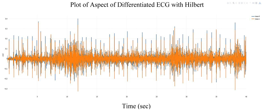
Fig. (1) below 40 second ECG signal derived from poly-somnography records provided by the National Sleep Research Resource (NSSR) [15], to illustrate QRS detection in this study.
Fig. (2) shows the ECG signal overlaid with the analytic signal (the Hilbert transform of the ECG signal). Fig. (3) shows the differentiated referenced ECG signal, which increases the noise but also tend to accentuate the peaks and Fig. (4) shows the differentiated referenced ECG signal overlaid with the analytic signal. In this case, the Hilbert transform of the differentiated ECG signal does not seem to offer a clear advantage for peak detection. However, since the Hilbert transform of a signal simplifies peak detection, the analytic signal of the differentiated ECG signal is used in this study.
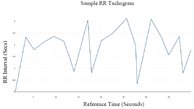
Subsequently, the R peaks can be located and an RR time-series tachogram of RR-intervals can be developed. A plot of the RR time series is shown in Fig. 5.



2.3. Sleep Episode Identification
Heart Rate Variability HRV characteristics will be used to differentiate between the Parasympathetic and Sympathetic Nervous Sub-system within the Autonomous Nervous System (ANS). The adopted method relies on the research by Hon et al. (1963) that revealed that HRV characteristics delineate specific ANS activity.
A frequency domain analysis of the RR time series using Fourier transforms for the power spectral analysis identifies a period of decreased heart rate as the range of epochs with (LF/HF < 1) which are also selected as the epochs within a sleep episode. In the case of this research, an explicit calculation of ratio in the frequency domain is avoided to mitigate errors due to the imperative style. Rather, a neural network is trained using correctly annotated sleep data to associate the frequency information of HRV data to time before sleep onset.
As mentioned, the RR interval series is transformed using Fourier Transform (FFT)
 |
(1) |
Where:
N = Number of samples in the time domain
n = Current number of samples considered
The magnitude of the signal is then calculated as follows
 |
(2) |
The power P(k) at X(k) is taken as the square of the magnitude
 |
(3) |
The frequency at X(k) is taken as
 |
(4) |
Fs is the sampling frequency.
k is the current frequency bin.
2.4. Sleep Potential Analysis
As mentioned before, the Sleep Potential (SP) is a measure of the time before the onset of sleep. Specifically, the Sleep Potential is a random variable that assigns a numerical value that encapsulates temporal information about the onset of sleep. In other words, a temporal value (measured in seconds) is assigned to the likelihood or probability of transitioning from “Awake” state to “Stage 1” sleep state.
The input data is the power spectral sequence of the RR “beat to beat” interval data, which is fed into a feedforward neural network as a (power, frequency, phase) pair. The neural network approximates the regression function whose output is a real number: f(g(X,Y,Z)) → φ
In a general sense, the input vector encapsulates the instantaneous or currently measured power, phase and frequency of a point in a “wake” power spectrum.
The Sleep Potential (SP) aspires to provide an instantaneous prediction of the time before a sleep episode which is known in this research as Time to Sleep (TTS).
A sequence of the [input: g(power,frequency, phase), output:TTS] is used to train a multi-layer neural network.
2.5. Architecture of the Sleep Potential Predictive Model
Neuron configuration by layer:
Layer 1: 3 Neurons
Layer 2: 10 Neurons
Layer 3: 20 Neurons
Layer 4: 1 Neuron
The choice of a multi-layer neural network was influenced by the perceived non-linearities or deviations observed in some of the samples in the training set, whose progression from the wake cycle to the sleep cycle does not adhere strictly to a linear decay of the LF/HF ratio of the RR (NN) beat to beat sequence. Another criterion for the presented network architecture is the speed of convergence. Fig. (6)
The neural network convergence was measured and recorded at an error tolerance level of 0.001 with a reference patient sample from the training dataset. Based on the combination of the factors described prior, the 3-layer neural network was adopted. The result of the convergence test is shown in Table 1 below:
| Trial | Layer 1 Neurons | Layer 2 Neurons | Layer 3 Neurons | Layer 4 Neurons | Convergence (Sec) |
|---|---|---|---|---|---|
| 1 | 4 | 5 | 10 | 1 | 39.6 |
| 2 | 4 | 10 | 20 | 1 | 4.1 |
| 3 | 4 | 20 | 40 | 1 | 7.6 |
| 4 | 4 | 20 | 20 | 1 | 44.49 |
2.6. Learning Algorithm: Resilient (Back)propagation
In general, Gradient Descent (GD) has wide applications in supervised learning but a heuristic adaptation known as Stochastic Gradient Descent is used in practice. This allows network weights and biases to be updated after every record or batch of records instead of after an epoch (the entire training set); this allows for shorter training time. Training is achieved when the cost of the gradient function is backpropagated through the network layers and weights are adjusted by computing the partial derivatives. The partial derivatives are artifacts of using Chain Rule to simplify the derivative of the cost function with respect to the weights.
The Resilient Backpropagation is used to accelerate convergence and reduce training time. It achieves this by rolling back weight updates when a significant change occurs (a process known as “backtracking”), increasing weight updates progressively which leads to faster convergence [11].
2.7. Activation Function: Bernoulli Function
The Bernoulli activation function is especially suitable for use as a stochastic activation function. It is a sigmoid neuron that is on or off based on an implicit probabilistic model that follows Bernoulli distribution. Stochastic activation functions are used in Dropout learning. The Dropout learning is a regularization technique where a neuron is “on” with a probability p or “off” (dropped out) with a probability 1 – p. This is very important in deep neural networks because it prevents overfitting, a situation where the neural network only learns to classify the training input or data instead of learning decisions boundaries [12].
3. RESULTS
A multi-layer neural network with the architecture described in section 2, is trained with a sequence of polysomnography electrocardiograms drawn from a set of patients over the age of 40. The patients lie in a broad range of health fitness; that is, some patients are in perfect health, while others may suffer from illnesses ranging from minor to more debilitating ones. The distribution of patients in this so-called health fitness spectrum is unknown. A sequence of feature vectors encapsulating the frequency domain characteristics as described in section 2 is obtained from all patients in the training and test sets. An assumption that the sequence of feature vectors corresponding to each patient is independent and uniformly distributed, that is, all feature vectors are equally likely. After training is complete, the model is tested on a test set of 105 patients. The output of the multi-layer neural network for predicting Time to Sleep (TTS) generally referred to as Sleep Potential (SP) is presented subsequently.
The test dataset consists of 10,000 seconds of 105 sleep episodes. The samples in the test dataset are independent of each other because they map to distinct patients. This notion of independence is also preserved in the training set. The samples in the training set were randomly chosen such that Q∩P= Ø for a set of training data Q, and test data P. The initial training set involved about 100 patients, randomly chosen with the goal of capturing the deviations or variance exhibited by the total population. For a good generalization of all possible progressions from a wake cycle to a sleep cycle considering frequency domain characteristics from training examples, we assumed by the rule of thumb we needed more than 30 examples. A practical consideration was made in this case not to strictly adhere to the 80/20 training-test data split, given the computational time complexity required for specialized pre-processing of data sampled at 125Hz, which means for every patient sample, there are 1.25 million feature vectors at the start before further pruning. The effective number of examples in the training set was varied iteratively until a perception of marginal improvement to the predictions in the test set were greatly diminished.
Every patient has a sequence of approximately10,000 feature vectors corresponding to the RR interval in the associated electrocardiogram. Half of these features are used in the test by selecting ones with even indices to reduce the number of data while retaining the distribution of feature vectors in the different sleep stages.
The goal is to predict the instantaneous Time To Sleep (TTS) using every feature vector and compare the prediction to what is recorded in the patient ECG annotations. Depending on the length of the wake cycle, the size of the predictions varies from patient to patient. Suppose a patient A, has 400 features in wake cycle and 4,600 features distributed through the sleep stages, the size of the predictions will be 400 because Time to Sleep (TTS) is only relevant in the wake cycle. Every feature vector in the wake cycle is fed in the neural network and value for TTS is obtained.
The overall result is presented in a compact way by recording a plot of the predicted TTS versus the actual TTS in the patient ECG annotations. The actual and predicted expected values (which in this case is the mean, since they are uniformly distributed) are recorded and tabulated for every patient. The recorded predicted and actual means is subsequently used to determine how well the predictive model replicates the true model.
A summary of the overall experiment is first presented as described for all test patients. A paired difference test (t-test) is used to determine the likelihood of observing the TTS data from the predictive model under the NULL hypothesis which is also the research hypothesis. Subsequently, the plots for every test patient are then shown.
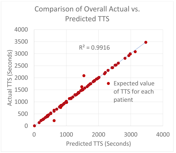
The figure below shows Fig. (7) the comparison of the TTS prediction (a measure of sleep onset latency) with the actual values obtained from clinical annotations of the test set. As expected, in most cases, the sleep onset latency predictions were very close to the observed values. The deviations observed are assumed to belong to patients who have endured a severe cardiovascular event, or may have assistive devices like a pacemaker or actively have congestive heart failure causing deviations in the recorded electrocardiograms which might have affected the quality of QRS detection, which in turn might imply an erroneous RR (NN) beat to beat sequence which if true, may lead to bad out of sample performance of those specific test data [16-19].
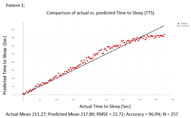
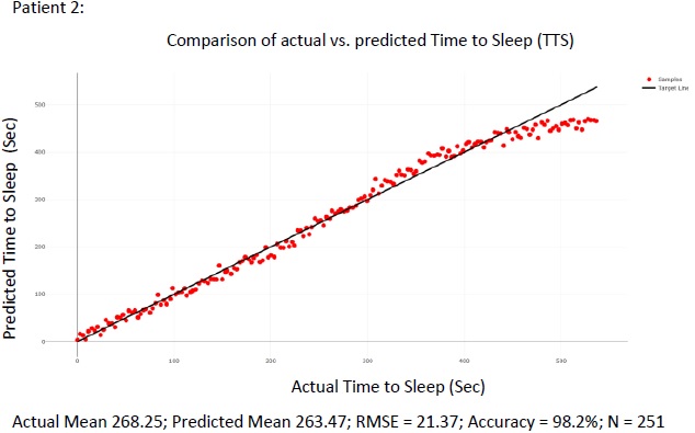
Also, the accuracy shown subsequently for the two example patients from the test set was computed as follow:
 |
The P-value = 0.976273 (which was calculated using a paired t-test of the measured and predicted values for all the patient in the test set). This means that the results confirm that we can improve on nominal scales of wakefulness used pervasively in sleep studies with a model with a better resolution of the distance relation (in terms of time) between an arbitrary point in the wake cycle and the onset of a sleep episode. These results also agree with Toscani et al., in 1996 and Busek et al. in 2005 who established that the LF/HF ratio decreases consistently from the wake cycle to the sleep cycle. The sleep cycle is delineated by an LF/HF ratio that is less than 1. This linear relationship makes it easy to model the ideal case. However, this behavior is not exhibited by the entire patients in the training set since they lie on different points on the health spectrum, as such this study extends the application of prior efforts by learning the non-linearities from examples that do not strictly follow the norm. For the healthy ones, the problem is trivial for a learning model which explains the high R2 values.
The figure above summarizes the error in the mean predicted Time To Sleep (TTS) and measures Time To Sleep (TTS) for all 105 patients in the test set Figs. (8 and 9) show. detailed results are presented for 2 of the patients in the test sets for the purpose of illustration. For each of the patient shown in the raw results, N points were selected from the wake cycle and TTS was predicted for each point. The mean value is reported as well as the Root Mean Squared Error (RMSE).
4. DISCUSSION
With the general usefulness of ambulatory ECG devices and the rise in wearable physiological process telemetry, this study paves the way for an integrated and continuous sleep awareness in a growing culture of fitness and general wellness.
This research has shown that it is possible to use quantitative data to predict the time to sleep. It has an advantage over the use of questionnaires for the diagnosis of sleep disorders since questionnaires often rely on the memory of the subjects. Therefore, a limitation is implicitly imposed on this type of method because memory is susceptible to biases and erodes over time; even heightened emotional states can distort the representation of information retrieved from memory. As such, introducing a reliable alternative to questionnaires in constructing sleep history helps in generating unbiased data for sleep disorder diagnosis and treatment. The methodology described in this research aspires to satisfy the prior stated goal of a reliable alternative to sleep history documentation and a general sense of awareness in the clinical prescription for sleep-related disorders using the proposed models.
However, the wakefulness indicator can be applied to other domains as well. An immediate application is the mitigation of the epidemic of drowsy driving. The reliance of the presented technology on easy to get ECG data, can cut down on the number of accidents related to drowsiness when operating vehicles or machinery requiring a high level of attention and focus for safe operation.
CONCLUSION
Investigating the use of machine learning to providing real-time insights into the inception of a sleep episode is the principal purpose of this research. This research affirms the notion that “Wake” and “Sleep stages” can be derived from analyzing ECG data. A demonstration of the possibility of forecasting time before sleep occurs during a wake cycle is also presented.
As expected, learning a statistical model to predict the realizations of a stochastic process is very dependent on the training set. In a general sense, it seems that for healthy patients, it was sufficient to model Sleep Potential (SP) as a function of frequency, and in others it was inadequate. From the correlation values obtained during feature analysis, it seems that at least 35% of the training set manifested some form of non-linearity. Consequently, it is important that the Sleep Potential (SP) multilayer neural network is able to learn the nonlinearities in the training set and performs really well on a test set with an unknown health distribution.
LIST OF ABBREVIATIONS
| SP | = Sleep Potential |
| TTS | = Time to Sleep |
| HRV | = Heart Rate Interval |
| MWT | = Maintenance of Wakefulness Test |
| DNN | = Deep Neural Network |
AUTHORS' CONTRIBUTIONS
All authors read and approved the final manuscript.
ETHICS APPROVAL AND CONSENT TO PARTICIPATE
This study was approved by the Texas Tech University IRB review process (IRB2017-455).
HUMAN AND ANIMAL RIGHTS
No animals / humans were used for the studies that are bases of this research.
CONSENT FOR PUBLICATION
Not applicable.
CONFLICT OF INTEREST
The authors declare no conflict of interest, financial or otherwise.
ACKNOWLEDGEMENTS
Declared none.

