All published articles of this journal are available on ScienceDirect.
Recognition Method of Limb Motor Imagery EEG Signals Based on Integrated Back-propagation Neural Network
Abstract
In this paper, in order to solve the existing problems of the low recognition rate and poor real-time performance in limb motor imagery, the integrated back-propagation neural network (IBPNN) was applied to the pattern recognition research of motor imagery EEG signals (imagining left-hand movement, imagining right-hand movement and imagining no movement). According to the motor imagery EEG data categories to be recognized, the IBPNN was designed to consist of 3 single three-layer back-propagation neural networks (BPNN), and every single neural network was dedicated to recognizing one kind of motor imagery. It simplified the complicated classification problems into three mutually independent two-class classifications by the IBPNN. The parallel computing characteristic of IBPNN not only improved the generation ability for network, but also shortened the operation time. The experimental results showed that, while comparing the single BPNN and Elman neural network, IBPNN was more competent in recognizing limb motor imagery EEG signals. Also among these three networks, IBPNN had the least number of iterations, the shortest operation time and the best consistency of actual output and expected output, and had lifted the success recognition rate above 97 percent while other single network is around 93 percent.
INTRODUCTION
Electroencephalogram (EEG) signals indicate the spontaneous and rhythmic electrical activity of brain cells contain enormous biological information and may reflect the physiological and psychological states of humans [1]. When people just imagine body movements but do not execute, the brain produces the same EEG pattern as the action performed. Thus we can use mind to control the external environment so as to achieve the action we thought by correctly and timely recognizing motor imagery EEG signals. But as the EEG signals belong to non-stationary ones, having characteristics of randomness, nonlinearity, being susceptible to disturbance for weak signals, etc. [2], there are many difficulties in the analysis of motor imagery EEG signals, especially for multi-class problems, and many classification methods are based on two kinds of motor imagery EEG signals for recognition. Nowadays, the recognition algorithm for motor imagery EEG signals is more focused on briefness, accuracy and celerity, which may make the human-computer interaction system to obtain the ideal recognition result within the shortest training time.
Currently, there are different methods for classifying the EEG signals. These methods, generally, could be categorized into two basic categories, one of which is called linear classification method and the other is called the nonlinear classification one [3]. The linear classification method contains Fisher linear classification method and the approximate entropy (ApEn) classification method; while the nonlinear classification method mainly includes the artificial neural network (ANN) and support vector machine (SVM) methods. Among the above methods, the ANN method is widely applied in various fields for its simple operation, strong adaptiveness and excellent prediction capability. These commonly used neural networks, however, may not ensure to well predict the new samples, that is to say that such networks are of poor generalization ability [4]. Moreover, factors of the sample size, parameter setting, distribution of training sets and testing sets, etc., may affect the calculation accuracy and operation time of ANN [5]. In order to avoid the influences of the above problems, and to improve the data recognition rate, this paper has proposed to research the limb motor imagery EEG signals by utilizing IBPNN.
Since Hansen and Salamon [6] first put forward the neural network ensemble (NNE) method in 1990, the neural network, after years of development, has been widely used in aspects of pattern recognition, risk prediction, etc. In 2008, Zhang Lei, et al. [7] used the integrated neural network in authenticating off-line signature and obtained the higher recognition rate. In 2012, Su C and Xiao NF [8] used the integrated BP network and received the higher recognition rate in face identification. In 2013, Lee H, et al. [9] also used the integrated neural network to recognize domain actions and got great recognition rate. Moreover, Qin LL, et al. [10] applied the integrated neural network in the modulation recognition of digital signals and such recognition rate was very high. Also referring to literatures [5] and [11], IBPNN has also been applied in recognizing electromyographic signals, and the result was very high. Thus it can be seen that the integrated neural network is popular in pattern recognition of many different fields and it has got great achievement. In this paper, the IBPNN is applied in recognizing the limb motor imagery EEG signals, which may quickly classify the EEG signals of three kinds of motor imageries so as to greatly shorten the operation time.
1. PRINCIPLES AND METHODS
1.1. Back-propagation Neutral Network
Artificial neural network (ANN) is a kind of data processing algorithm established through simulating the brain neural network features, having strong learning ability and adaptability [12]. There are many types of ANNs, such as BPNN, Elman neutral network, learning vector quantization (LVQ) neutral network, and the wavelet neutral network (WNN) [13-16]. The BPNN algorithm, however, is one of the relatively mature algorithms, and belongs to the multilayer forward neural network. Mutual propagation among neurons is by the way of Sigmoid functions, and BPNN can actualize any nonlinear mapping from input to output. The learning process of BPNN can be divided into two parts - positive propagation and back propagation. Fig. (1) has shown the structure of three-layer BPNN. The number of neurons in input layer is n, hidden layer neurons with q and m for output layer. The connective weight between the input and hidden layers is w, as v is such connective weight for hidden and output layers. In addition, the threshold value of hidden layer is b while such value for output layer is t, and we have taken it as an example to explain its operational principle.
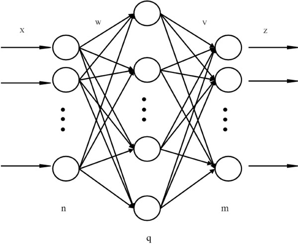
Structure of Three-layer BPNN.
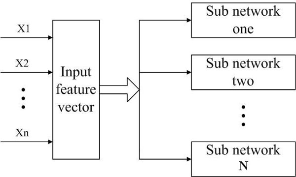
Structure of IBPNN.
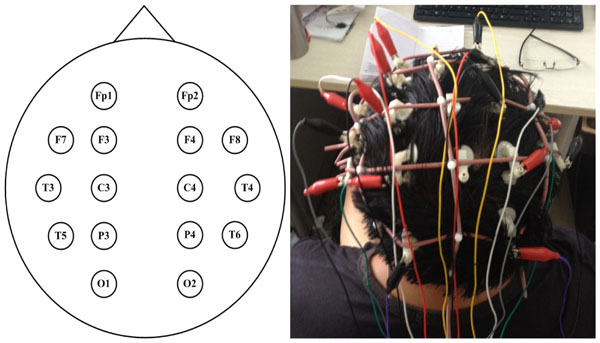
Locations of Electrodes.
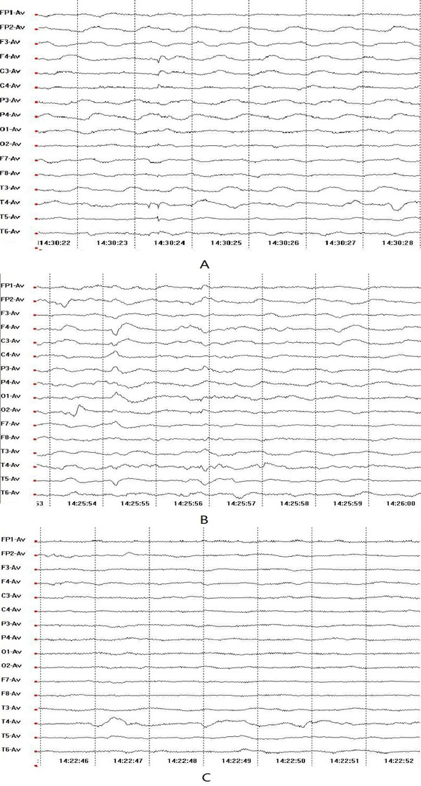
Raw EEG Signals of Different Motor Imageries. (A: Left-hand Movement Imagery; B: Right-hand Movement Imagery; C: No Movement Imagery.)
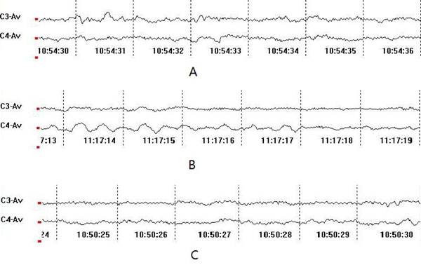
Filtered EEG Signals of Different Motor Imageries at C3 and C4.(A: Left-hand Movement Imagery; B: Right-hand Movement Imagery; C: No Movement Imagery).
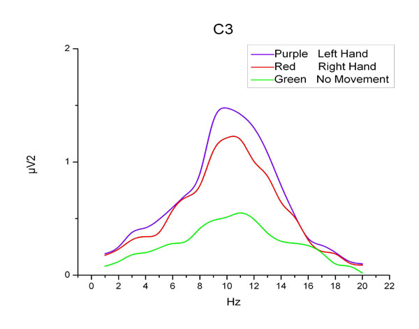
Energy Spectrum Density Curves at C3.
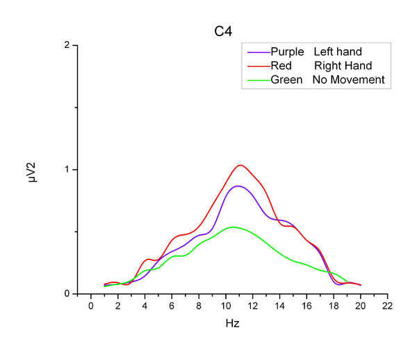
Energy Spectrum Density Curves at C4.
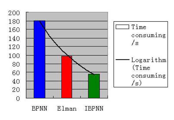
Consuming Time for Three Networks.
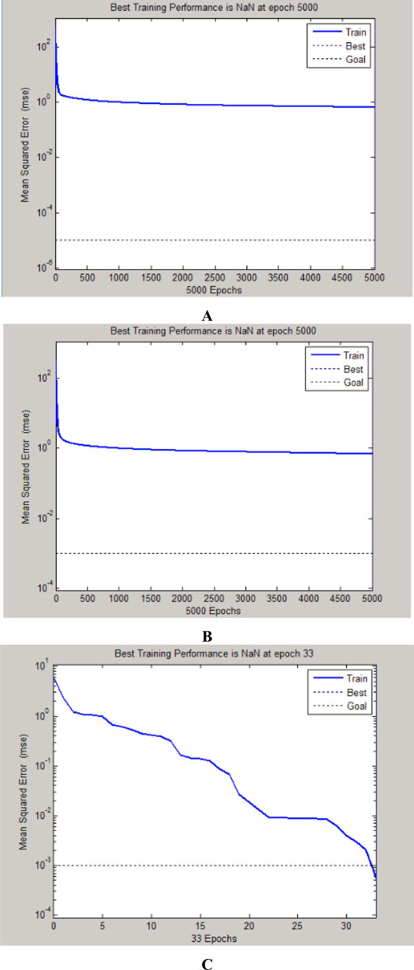
Iterations and MSE of Each Neural Network. (A: BPNN; B: Elman Neural Network; C: IBPNN).
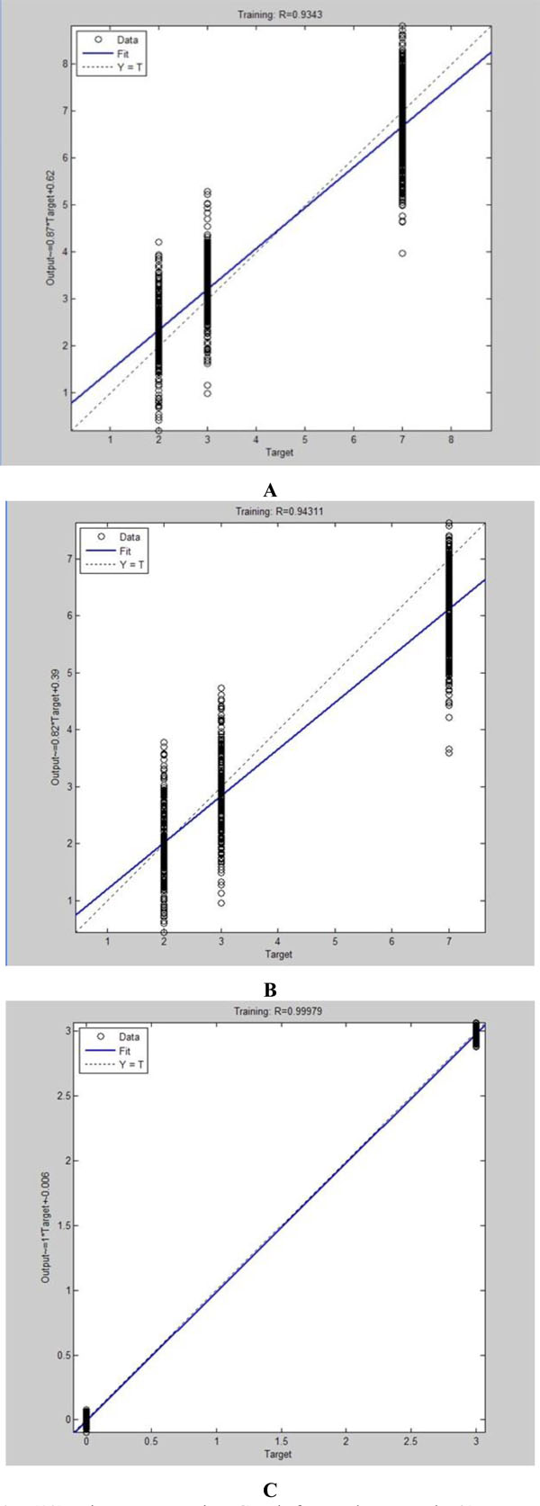
Linear Regression Graph for Each Network. (A: BPNN; B: Elman Neural Network; C: IBPNN).
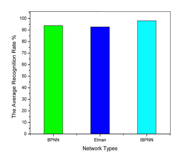
Average Recognition Rate of Each Network.
1.1.1. Positive Propagation
Positive propagation, also a process of sample learning, is to operate backward for output through the previous weight and threshold. Supposing a given feature vector , the input and output of the hidden layer is respectively as follows:

 (1)
(1)

 (2)
(2)
Where the input of hidden layer is h, the output of hidden layer is o, and the activation function of hidden layer is f (.). The output of the hidden layer would continue propagating forward to the output layer. Thus the input and output of the output layer is respectively as follows:

 (3)
(3)

 (4)
(4)
Where the input of output layer is y, output of output layer is z, the activation function of output layer is . Then comparing z with the desired output, the network will determine whether to conduct the back propagation.
1.1.2. Back Propagation
Back propagation is the error one as well. The weight factors and threshold value of each layer would be adjusted according to the output error operated from output layer to the next one, if the actual output and the expected value do not match. Formula will be workable if the error function for the Kth sample is e. Error function is used to adjust the weights of each layer. The weight adjustment formulas of input and hidden layers as well as hidden and output layers are as follows:


 (5)
(5)


 (6)
(6)
Where  is learning rate,
 is the partial derivative of error
function for every neuron input of hidden layer, and
 is
the partial derivative of error function for every neuron input of output
layer.
The two stages are repeated alternately, and the network training will end until the networks converge to an ideal state or the learning times reach the preset limit. In this way, the network may be used in actual recognition. From the two working steps of a single BPNN, we can know that its neural nodes for output layer correspond to the predetermined action classes, while in the process of pattern recognition, these neural nodes are fixed, so the classifier is easy to generate local minima, requiring a sufficiently large training set to recognize the input feature vectors correctly in the text stage [5].
1.2. Integrated Back-propagation Neural Network
Neural network ensemble is to learn a common issue with a finite number of neural networks, and the output of ensemble under certain input example will be jointly decided by output of various sub networks constituting such ensemble under this example [17]. The integrated neural network can improve the generalization ability of network so as to improve the accuracy of pattern recognition [11]. Reference [8] has proved that compared with the single network, the integrated network combined with several simple sub-networks may get more stable and efficient classifiers in a shorter period of training time. Thus in this paper, the IBPNN designed is composed of multiple single BPNNs, and these sub-networks are not connected with each other. The reason why these sub BPNNs should be independent is that the sub networks are more likely to fall into disparate local minima to improve adaptability for data untrained previously. The parameters of each network, such as the number of nodes, learning rate and accuracy of training are adjustable to the actual situation, thus IBPNN is more appropriate for the diverse and multiple data sets instead of the unitary parameter settings of a single network. And, every neural network is only responsible for recognizing one class of data, which is equivalent to simplify the problem. In this way, every sub BPNN is more specific and stable. Each sub BPNN recognizes one kind of data exclusively and they execute at the same time. So IBPNNs cannot only guarantee the accuracy but also can shorten the operation time. The structure model for BPNN could be described as Fig. (2).
The working process of IBPNN is as follows:
(a) Learning
samples and completing the parameter adjustment for the network. We set the
number of sub BPNN as S as the sample contains S types of data. The Network k
is in charge of the data type k (  ). The output of
each sub-network has only two states of either 1 or -1. Only the expected
output of data which is related to corresponding network will be set to 1,
otherwise will be set to 0. Then we put the training sample into the integrated
network. At the training stage, the network adjusts its weights and biases and
variable parameters so as to capture the relationships between the input
patterns and outputs [18]. After all sub BPNNs reach the certain accuracy, the
training action ends;
(b) The classification of actual data. Input the testing set into the IBPNN trained. If the output of the sub-network k is the largest, the data will be categorized as k.
2. PATTERN RECOGNITION EXPERIMENT FOR LIMB MOTOR IMAGERY EEG SIGNALS
2.1. Data Collection of EEG Signals
In this paper, the data of EEG signals is measured by the 16-channel SOLLAR1848 digital electroencephalograph manufactured by Beijing Solar Electronic Technologies Co., Ltd. while performing the three limb motor imageries (imagining left-hand movement, imagining right-hand movement and imagining no movement). Our subjects are three healthy postgraduates at the age of 24 and their mental states are stable. As the EEG signals are unstable, subjects need to receive meditation training to guarantee the accuracy of the measured data. We test for 6s for each imagery. And signals we received will be preprocessed by the instrument software. Since these subjects will take some time to round into imagination, we take the data of 2s-5s as analysis information. 200 groups of data are collected from one subject for one kind of motor imagery. And Fig. (3) has displayed the locations of these electrodes.
2.2. Feature Value Extraction of EEG Signals
In order to correctly recognize different EEG signals, we should extract values being suitable and characteristic as input values. And the difficulty of pattern recognition increases with the number of mental tasks [19]. So the feature value extraction is a key link for the classification. Whether the feature value is appropriate or not will seriously affect the accuracy of recognition. However, it is tough for researchers to extract feature values from EEG signals as the amplitude for EEG signals is small, such signals are vulnerable to be interfered, etc. Consequently, feature value extraction is a hot issue that many researchers focus on. As features of EEG signals on the frequency domain are more obvious, the frequency domain analysis technology is a common method for extracting feature values of EEG signals. The law of EEG signals varying with frequency will be reflected by features such as amplitude, phase spectrum, power spectrum and energy spectrum [20]. As an important feature for EEG signals, Energy is not only physiologically rational but also empirically effective [21]. So we adopt energy as the feature of EEG signals. In this paper, we take advantage of frequency analysis to extract feature vectors of different motor imagery. Applying Fourier transform on the signal allows the frequency content to be obtained [22]. Get the average energy at each electrode of EEG signals, and then gather the data as the input vector. And every set of feature values for limb motor imagery EEG signals is produced by this way.
The raw EEG signals of three motor imagery at each electrode measured in this paper is shown in Fig. (4).
During the data collection process, EEG signals are apt to be interfered by instruments, so the collected data usually mixes with some interferences, which lead to low signal-to-noise ratio (SNR) [23]. In order to extract such EEG signals exactly, the interference signals must be filtered out by the band-pass filter (8-20Hz). We use the data at C3 and C4 for analyzing and selecting the obvious frequency range as integral interval, as C3 and C4 electrodes are located in the center of the movement area managed by the left and right brains respectively. These three pictures in Fig. (5) have displayed the EEG signals filtered of different motor imageries at C3 and C4.
We first deal with the signals by Fourier transformation, and then acquire the power spectrum density. In this way, we may gain the energy spectrum density curves of three motor imageries at C3 and C4 shown in Fig. (6) and Fig. (7). We can see from these pictures that, the three curves of C3 electrode should be distinguished clearly at 7-15Hz, while the curves at C4 is different at 8-14Hz. So we take the overlap (8-14Hz) from two frequency ranges as the selected frequency band. Totally there are 16 channels in experiment and we compute the integral of energy density at each electrode within 8Hz to 14Hz. And the integral formula can be written as:
 (7)
(7)
In equation (7), St is the corresponding energy for the specific channels, stands for the function of energy spectrum density, and f2 and f1 are separately the upper and lower limits of the integral.
Thus the feature value is composed as:
 (8)
(8)
Where Di is defined as the feature vector corresponding to the data set i.
2.3. Design of IBPNN Classifier
Compared with the single network, IBPNN has better fault tolerance and generalization. And the trait of distributed computing will greatly shorten the training time. BPNN with individual hidden layer could map all functions [24]. So we chose the three-layer BPNN as sub-network in this paper. As the EEG data to be recognized may be divided into three sets, and the number of sub-network is set to three, NET 1 is adopted to recognize the right-hand imagery data, while NET 2 and NET 3 are separately designed for recognizing left-hand and standing imagery data. The input vector for each sub-network has 16 nodes and two states will be output, thus 16 nodes are set for the input layer, while the output layer has with two nodes.
The number of hidden layer is
determined by experience and speculation, and the equation
 may be referred. Where a represents for any constant between 1-10. So
by referring to the above equation, the range of hidden layer nodes for
integrated BP network should fall in [8, 21]. By combing this range, we carry
out trails to find the optimum node number of hidden layer for sub-networks
according to its relevant data types. After experiment, the parameters for
hidden layer are set as Table 1.
2.4. Algorithm Process for Motor Imagery EEG Signals
Node number of hidden layer for each sub-network.
| Network No. | NET 1 | NET 2 | NET 3 |
|---|---|---|---|
| Number of Nodes for Hidden Layer | 10 | 7 | 5 |
Data distribution of training testing sets.
| Motor Imagery | Training Set | Testing Set | Total |
|---|---|---|---|
| Right-hand | 300 | 300 | 600 |
| Left-hand | 300 | 300 | 600 |
| No movement | 300 | 300 | 600 |
Recognition Rate of Different Motor Imageries.
| Motor Imagery | BP (%) | Elman (%) | IBPNN (%) |
|---|---|---|---|
| Right-hand Left-hand No movement |
92.62 93.18 91.73 |
93.45 92.12 92.56 |
98.57 98.32 97.14 |
This paper uses MATLAB to write the IBPNN program, and the algorithm implementation steps are shown as follows:
a) Read the training and testing sets data from M files;
b) The data was normalized so that the element value of every feature vector is in (0, 1), which is convenient for computing and adjusting the networks;
c) Data computed by process b) should be put in IBPNN for classification;
d) Output the weights and thresholds of various sub-networks and write them into Mat files for saving;
e) Display the data numbers being correctly recognized, and calculate the success classification rate.
3. EXPERIMENTAL RESULTS AND ANALYSIS
In order to more intuitively reveal the superiority of IBPNN, in this paper, we have not only adopted the individual BPNN as comparison set, but also designed the Elman neural network algorithm for adding the accuracy of this experiment conclusion. Operation time, number of iterations, imitative effect and success recognition rate are compared to develop the most effective classifier among these three networks.
First we should distribute the EEG signals of three motor imageries for training and testing sets according to the feature values. Sample size of the training set should not be too small, otherwise the neural networks may not have a good knowledge of the rules and relationships contained in the samples during the learning process; meanwhile, there shall not be too many samples, which, otherwise, may incur more training time. In the experiment of this paper, it turns to be suitable for setting 300 as the number of training set by experiments, which may stabilize the training effect and ensure the reasonability of such training time. In this way, we have taken randomly 100 sets of data from 200 sets of set of actions made by each subject, and the rest data may be as the testing set. In the end, for one kind of motor imagery, training and testing sets contain 300 sets of vectors respectively. And the data distribution is shown in Table 2.
Train and test the data. We can see from Fig. (8) that, for operating 1800 sets of data, the individual BPNN needs 181s and the Elman network consumes 98 s. However, the three sub-networks of IBPNN consume only 56 s in total when accomplishing the operation. Hence we can come to a conclusion that the operation time of IBPNN is the shortest.
We can also know from the analysis of iterations and the mean square error (MSE) that, the result for IBPNN is also satisfying. The IBPNN reaches the setting error 0.001 at the thirty-third times of iterations while the other two do not until the number of iteration arrive to pre-determined limits 5000. Fig. (9) has shown the iterations and MSE from three different neural networks.
Fig. (10) is the linear regression graph for each network. Linear regression is used to explain the tracking condition of desired output. On behalf of fit goodness, R ranges from 0 to 1. For IBPNN, its actual output is more approximate to the expected output as R is closer to 1. However, the fitness of other two networks is not ideal.
The recognition rate is the important index for determining the recognition effect of the various neural networks. The recognition rate in this paper may be operated by the following equation:
 (9)
(9)
Where p stands for the success recognition rate, R is the number of vectors being correctly recognized, and N is the total vectors. Referring to the above equation, we obtain the recognition rate for the EEG signals of there motor imageries, as is demonstrated in Table 3. And the average recognition rate of each network is revealed in Fig. (11). By comparing either the average rate for each network or the recognition rate for single action, we can see from Fig. (11) and Table 3 that IBPNN is better than BPNN and Elman networks. The average classification rate of IBPNN is 98.01% which is much more than BPNN and Elman network.
4. DISCUSSIONS
In this paper, we have mainly conducted the pattern recognition for EEG signals based on three different motor imageries by utilizing the method of IBPNN, and we have also contrasted IBPNN with BPNN in four aspects of iterations, operation time, the consistency of actual output and expected output, and the success recognition rate. The experimental results has shown that, when the data categories reach three, the correct recognition rate of IBPNN is significantly higher than that of a single neural network, and the operation speed is faster as well. The IBPNN overcomes the problems of low generalization, intricate scale as well as long operation time for BPNN. Therefore, IBPNN is more competent in recognizing EEG signals of motor imageries.
The IBPNN is composed of several sub-networks, which are independent from each other. Thus each sub-network has its own proper job and may not be influenced by other ones. In the training stage for networks, each sub-network has to achieve one relationship from input to output, and then the structure and training process of sub-networks will be simplified. With these characteristics, IBPNN cannot only enhance the advantages of sub-networks, but also may reduce the weakness of it.
Due to the specificity of these EEG signals, we cannot guarantee the accuracy of every set of data. Therefore, the rate for IBPNN recognizing EEG signals is not perfect. Moreover, IBPNN itself has certain limitations as well; there is lack of theoretical basis for the choice of neurons in hidden layer, what’s more, the initial weights and thresholds for networks are acquired randomly. The recognition rate of motor imagery EEG signals may also be influenced by the above-mentioned limitations. In our future work, therefore, we will design a BCI system based on IBPNN while improving the IBPNN algorithm, so as to get a friendlier environment for human-computer interaction.
ABBREVIATIONS
CONFLICT OF INTEREST
The authors confirm that this article content has no conflicts of interest.
ACKNOWLEDGMENTS
The authors gratefully acknowledge the financial supports from the specialized research fund for doctoral program of Chinese University (20100061110029) and the important development project of Jilin Province, China (20090350).

