All published articles of this journal are available on ScienceDirect.

A Numerical Simulation using Efficient, Parallel Computing to Model the Effects of Mechanical Properties of the Arterial Wall and the Frequency of Pulse Waves on Pulse Waveforms and Wall Shear Stress Distribution
Abstract
Background
Atherosclerosis is a risk factor for ischemic heart disease, and its progression has been associated with wall shear stress (WSS). While pulse waveform analysis has garnered increasing attention as a diagnostic indicator for atherosclerosis, the influence of the mechanical properties of arterial walls and the frequency of pulse waves on the pulse waveform and wall shear stress distribution has not been completely elucidated.
Methods
In this study, three-dimensional fluid-structure interaction analysis was used to simulate the pulse wave propagation phenomena in the aorta. The effects of the mechanical properties of the arterial wall and the frequency of the pulse waves on the wall shear stress distribution and pulse wave dynamics were investigated.
Results
In the investigation of wall shear stress distribution, under conditions of low Young’s modulus or high frequency, the time-averaged wall shear stress (TAWSS) was low and the oscillatory shear index (OSI) became high. In contrast, under conditions of high Young’s modulus or low frequency, TAWSS was high and OSI became low. In the pulse waveform analysis, the influence of viscous friction incorporated in the three-dimensional fluid-structure interaction analysis confirmed that the pulse waveform attenuated and diffused during propagation. A causal relationship between the TAWSS values and the attenuation or diffusion of the pulse waveform was not observed.
Conclusion
These results suggest that changes in arterial wall properties and differences in pulse wave frequency significantly influence WSS distribution. Furthermore, viscous friction in the three-dimensional FSI simulation led to attenuation and diffusion of the waveforms. However, the accuracy of waveform separation was insufficient, highlighting the need for improved methods that consider three-dimensional effects.
1. INTRODUCTION
According to the World Health Organization, ischemic heart disease was the leading cause of death worldwide in 2021 [1]. Atherosclerosis is characterized by abnormalities such as arterial wall thickening, decreased elasticity, or the development of stenosis. Because of the lack of subjective symptoms, the early detection of atherosclerosis is crucial. Currently, ultrasonography is the primary method for geometrical diagnosis of atherosclerosis [2]. However, ultrasonography is expensive and requires large-scale equipment, which means it may not always be suitable for the early detection of atherosclerosis. Consequently, diagnostic methods based on pulse wave propagation phenomena have been investigated as a simpler and more cost-effective alternative. Atherosclerosis is a risk factor for ischemic heart disease and involves the formation of atherosclerotic plaques on the inner surface of arteries, which eventually obstructs blood vessels and causes the functional decline or arrest of vital organs [3]. The preferred sites of atherosclerotic plaques, such as the carotid or radial arteries, suggest that the development of atherosclerosis may be related to hemodynamics. Giddens et al. reported that longitudinal shear stress remains within a range of 1 to 2 Pa in human coronary arteries [4]. Caro et al. proposed the low-shear hypothesis, which suggests that in regions of low wall shear stress (WSS), blood flow stagnation allows lipids and other substances to penetrate the arterial wall, leading to the formation of atheroma [5]. Furthermore, Ku et al. defined the oscillatory nature of WSS over a pulsation cycle as the oscillatory shear index (OSI) [6]. Dai et al. analyzed WSS waveforms and reported that waveforms with low time-averaged WSS (TAWSS) and high OSI promoted the development of atherosclerosis [7]. In addition, Fukui et al. reported that the motion of the arterial wall influenced the distribution of WSS [8]. In recent studies, Kumar et al. conducted a three-dimensional fluid-structure interaction analysis of the human carotid artery with a stenosis at the origin of the external carotid artery [9]. They observed regions of low WSS under conditions of high peripheral vascular resistance, suggesting a relationship with the progression of atherosclerosis. Cox and Plesniak investigated, in an arterial model with a bend, how differences in the inlet velocity distribution affect secondary flows and the WSS distribution [10]. They indicated that under fully developed inlet boundary conditions, complex secondary flows occur, resulting in higher OSI and increased morbidity. Although many studies have focused on boundary conditions, the impact of mechanical properties of the arterial walls on the WSS distribution has not been completely elucidated.
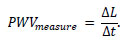
Pulse wave propagation refers to the vibration of the arterial wall caused by the contraction of the heart, which propagates blood flow to the peripheral regions. During propagation, physical phenomena, such as attenuation and reflection, occur due to the arteries’ geometric and mechanical properties. The propagation speed of the pulse waves, known as the pulse wave velocity (PWV), is obtained in vivo by dividing the distance ΔL between two measurement points by the time delay of the waveform Δt.
Therefore, Eq. (1) is as follows:
 |
(1) |
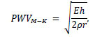
Thus PWVmeasure is obtained as the average speed between the two measured points. The Moens-Korteweg Equation [11] is often utilized to evaluate PWVmeasure. Eq. (2) expresses the PWV as follows.
 |
(2) |
where E is the Young’s modulus of the arterial wall, h is the wall thickness, ρ is the blood density, and r is the inner radius of the artery. Based on this equation, it is predicted that changes in the mechanical properties of the arterial wall, such as thickening, decreased elasticity, or atherosclerosis-associated stenosis, will lead to an increase in PWVM-K. However, the Moens-Korteweg equation is derived under many idealized assumptions that substantially deviate from the actual geometric and mechanical environment of biological systems. Therefore, diagnosing atherosclerosis using PWVmeasure based on PWVM-K raises some concerns regarding its reliability. Furthermore, PWVmeasure only evaluates the velocity of the wave propagation and does not account for the biological information contained within the pulse waveforms. Therefore, to establish PWVmeasure as a more reliable diagnostic indicator, “pulse wave analysis,” which considers the dynamics of the pulse waveforms, has garnered attention. Using the property of wave reflection at impedance discontinuities, such as arterial branches or stenoses it may be possible to extract geometric and mechanical information about the arteries from the pulse wave dynamics [12]. Parker and Jones proposed a method to separate the pulse waveforms into forward and backward waves and further analyzed the wave intensity, which represents the energy flux carried by the waves [13]. Fukui et al. indicated that reflected waves from stenosed and aneurysmal arteries differ in phase and that the geometric properties of the lesion itself influence the waveform of the reflected waves [14]. In recent studies, Khir et al. investigated arterial models with tapered structures and reported that the tapering angle affects the pulse pressure waveforms and the intensity of reflected waves [15]. In addition, Wu and Zhu examined arterial models with tapered structures and investigated the effects of variations in wall properties and physiologically relevant outlet boundary conditions on input impedance and reflection coefficients [16]. Both studies were conducted using one-dimensional analyses, and there are few studies that have performed waveform analysis using three-dimensional methods. Therefore, the objective of the present study was to simulate the pulse wave propagation phenomena in the aorta using three-dimensional fluid-structure interaction analysis to investigate the dynamics of the pulse waveforms and the distribution of the WSS with different Young’s modulus of the arterial wall and frequency of inflow velocity.
2. METHODS
2.1. Computational Models
To simulate the pulse wave propagation phenomena, a three-dimensional straight cylindrical model of the aorta, as shown in Fig. (1), was used for fluid-structure interaction (FSI) analysis. FSI is a method for analyzing the interaction between fluids and structures, enabling the investigation of the effects of blood flow on the arterial walls and the influence of arterial wall deformation on blood flow. Analyzing the detailed distribution of wall shear stress (WSS) and the deformation behavior of the arterial wall, in a manner that reflects the in-vivo vascular environment, is challenging in experimental studies or one-dimensional analyses. However, by performing FSI analysis, these aspects can be examined in detail. The outer part of the model consisted of solid elements simulating the arterial wall, while the inner part was composed of fluid elements simulating the blood flow. Hexahedral elements were employed for meshing, with the solid domain consisting of 256 elements and the fluid domain consisting of 704 elements at one cross-section. According to the resolution verification, the axial grid length dl was determined to be 2.5 mm. The average wall thickness of the human aorta is approximately 2 mm, with an inner diameter of approximately 13 mm [17]. In this study, to satisfy the assumptions of the Moens-Korteweg equation, such as a “sufficiently thin wall” and “infinitely long tube,” the inner diameter was set to r = 20mm (10 times as large as the wall thickness h), and the axial length was set to L = 3,000mm (150 times as long as the inner diameter r). Fukui et al., estimated the mechanical properties of arterial walls via in vitro biaxial tensile test [18]. Based on this study, previous research set the arterial wall’s Young’s modulus in numerical analysis [19]. In this study, following these prior investigations, the Young’s modulus of the arterial wall was set to three different values (E = 0.5, 1.0, and 1.5 MPa) corresponding to different stages of atherosclerosis progression, which are characterized by the accumulation of plaque inside the arteries and the resulting decrease in arterial wall elasticity.
The Poisson’s ratio and initial density of the wall were set to v = 0.45 and
 = 1,000kg/m3 , respectively. The blood was modeled as a viscous fluid with a kinematic viscosity of v = 4.0 x 10⁻⁶m2/s, a speed of sound of C = 100 m/s, and an initial density of
 = 1,000 kg/m3.
Additionally, this study enhanced the computational efficiency through parallel computing. The specifications of the PC used for the simulations are Intel Xeon Gold 6538Y+: number of cores, 64; memory size, 512 GB. The analysis solver RADIOSS used in this study features highly efficient parallelization capabilities. Fig. (2) shows that computational efficiency improved linearly with 1 to 8 parallel processes. However, from 16 to 32 parallel processes, the clock frequency dropped, diminishing the benefits of parallel computing. Therefore, in this study, computations were performed using 16 parallel processes.
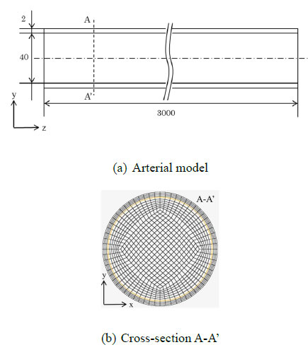
(a) Arterial model used for the simulations. (b) Cross-section of the arterial model.
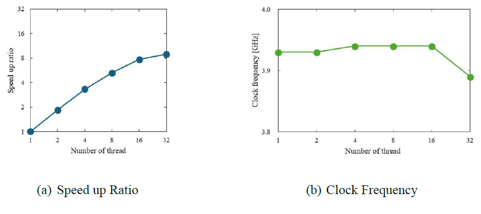
(a) Speed up ratio with increasing number of threads. (b) Clock frequency at each number of threads.
2.2. Governing Equations
In this study, the nonlinear structural analysis solver, RADIOSS (version 2022, Altair), was used to perform the FSI analysis. RADIOSS is an explicit finite element analysis solver, which is well-suited for high-precision analysis of dynamic motions such as pulse wave propagation and rapid deformation of the arterial wall. Additionally, the Arbitrary Lagrangian-Eulerian formulation was employed to analyze the movement of the fluid-solid interface. This approach enables accurate tracking of mesh variations associated with arterial wall deformation and high-precision analysis of the interactions between blood flow and the wall. The governing equations for the fluid domain included the conservation of momentum Eq. (3) and conservation of mass Eq. (4) [20].
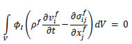 |
(3) |
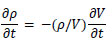 |
(4) |
Here, φI represents the weight functions, pf is the material density,
 is the velocity,
 is the stress matrix, and V is the volume.
The fluid was modeled as a viscous material using the following Eqs. (5 and 6).
 |
(5) |
| P = Bµ | (6) |
Here, Sij is the deviatoric stress tensor, eij is the deviatoric strain tensor, v is the kinematic viscosity, and P is the pressure. The bulk modulus B and μ were calculated using the initial density
, and the speed of sound c, as per the following equations Eqs. (7 and 8).
 |
(7) |
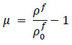 |
(8) |
For the structural domain, the equilibrium Eq. (9) was used.
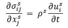 |
(9) |
The superscript s indicates the solid domain. The structure was modeled as a linear elastic material using the following constitutive Eq. (10).
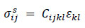 |
(10) |
Here, Cijkl is the elasticity tensor, and Ɛkl is the strain tensor.
2.3. Boundary Conditions
At the interface between the fluid and structural domains, a no-slip condition was applied, thereby ensuring that the velocities of the two components on the wall were equal, as expressed by Eq. 11.
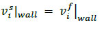 |
(11) |
In addition, both ends of the structural domain were fixed for displacement and rotation, as expressed by Eq. 12.
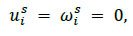 |
(12) |
where ω represents the angular velocity.
As shown in Fig. (3), at the fluid inlet boundary, a steady and uniform flow perpendicular to the cross-section was initially applied to develop the flow. Subsequently, a single sinusoidal wave with a specified period of λ was introduced to generate a compression wave and produce a single pulse wave caused by the vibration of the arterial wall. In vivo, pulse waves are composed of multiple sinusoidal waves with periods ranging from approximately 100 to 1000 ms (including waves corresponding to the heart rate, naturally occurring arterial vibrations, and their reflected waves) [21]. In this study, to investigate the effects of the pulse wave frequency on the waveforms and WSS, three different periods (λ = 125,250, and 500 ms) were used. At the fluid outlet boundary, a zero-pressure Dirichlet boundary condition was applied for the generation of reflected waves due to impedance mismatches in actual blood vessels.
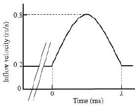
Inlet boundary conditions.
2.4. Separation of the Pulse Waves
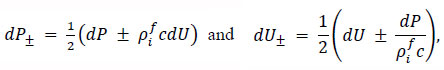
When the pulse wave reached the outlet boundary, the impedance mismatch between the outlet side and the preceding side generated reflected waves, which interfered with the incident waves. In this study, the separation of the pulse waves was performed according to the method proposed by Parker and Jones to investigate the effects of the mechanical properties of the arterial wall and the frequency of the pulse waves on the incident waveforms [13]. This method uses the property that the phase of the reflected wave differs by 180° between the pressure and velocity pulse waves. The incident and reflected components of the pressure dP± and dU± velocity pulse waves were expressed using the following Eq. (13).
 |
(13) |
where the incident wave is denoted by the subscript +, while the reflected wave is denoted by the subscript -. The wave velocity c was calculated using the phase velocity method based on the velocity pulse waves observed at z = 1,450 and 1,550 along the arterial model [15].
2.5. Calculation of the Pressure
In this study, the pressure applied to the inner artery wall was derived from the radial displacement of the arterial wall Dr .
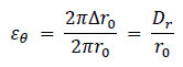
Using the initial radius of the arterial wall r0, the circumferential strain caused by the wall expansion can be expressed as follows Eq. (14):
 |
(14) |
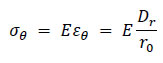
According to Hooke’s law, the circumferential stress acting on the wall σθ is given by, Eq. (15)
 |
(15) |
For a thin-walled cylindrical structure with a wall thickness h, the circumferential stress σθ can also be expressed in Eq. (16) using the internal pressure p as follows:
 |
(16) |
Combining these Eqs. (15 and 16), the pressure applied to the inner wall of the artery can be calculated as
 |
(17) |
2.6. Calculation of the WSS
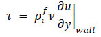
In this study, blood was assumed to behave as a Newtonian fluid, and the WSS was calculated using Newton’s law of viscosity Eq. (18):
 |
(18) |
The velocity gradient near the wall was determined based on the velocity values at three points in the normal direction, using a second-order Lagrange interpolation polynomial. In addition, the radial motion of the wall caused by the pulse wave propagation was taken into account during the calculations. The TAWSS over one pulsation cycle and the OSI, which quantify the variation in the magnitude and direction of the WSS over time, Eqs. (19 and 20) were calculated as follows:
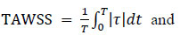 |
(19) |
 |
(20) |
2.7. Summary of Methods
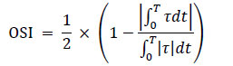
RADIOSS was used to perform pre-processing and computation, after which post-processing was carried out. A flowchart illustrating this workflow is shown in Fig. (4).
3. VALIDATION
To verify the numerical reliability of the analysis solver RADIOSS and the physical validity of the computational model used in this study, a comparison with previous studies was conducted [19].
The computational model employed a three-dimensional straight cylindrical model, as shown in Fig. (1). In comparison with previous studies, the inner diameter was set to r = 10mn and the axial length was set to L = 1,000mm. The Young’s modulus of the arterial wall was set to three different values (E = 0.5,1.0,1.5,2.0 MPA). The period of the inlet velocity was set to λ = 20ms. The other conditions were the same as those in Section 2.1.
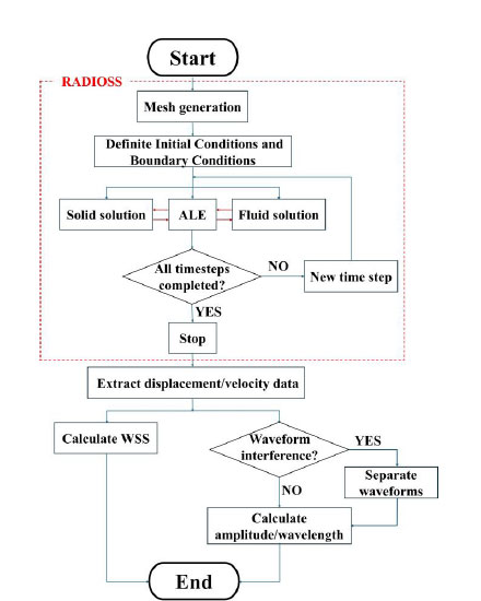
Fig. (5) shows PWVmeasure at z = 500 mm for each Young’s modulus and the PWVM-K calculated from the Moens-Korteweg equation. Additionally, Table 1 presents the error between PWVM-K and PWVmeasure for each Young’s modulus. PWVmeasure was calculated using the phase velocity method [22]. This method involves shifting one of the observed pulse waveforms at two measurement points, aligning the foot of the waveforms, and measuring the distance moved as the time delay ∆t. PWVmeasure was then calculated using Eq.(1). At the location z = 500mm, the local PWVmeasure was determined from the two waveforms at z = 450mm and 550 mm. The results indicate that, for all Young’s modulus values, PWVmeasure was estimated to be lower than the theoretical value. Furthermore, as the Young’s modulus increased, the error between PWVmeasure and PWVM-K also increased. This trend is due to the compressibility of the fluid. Although the Moens-Korteweg equation does not account for fluid compressibility, the fluid in this study was set to a slight compressibility. Consequently, discrepancies arose between the theoretical values and the numerical solutions. In particular, as Young’s modulus increased and PWV approached the speed of sound in blood (C = 100 m/s), the influence of compressibility became more pronounced, resulting in larger errors. These results are consistent with the trends reported in previous studies [19], thereby confirming the physical validity of both the RADIOSS solver and the three-dimensional straight cylindrical model.
Flowchart showing pre-processing to post-processing of simulations.
The effect of Young's modulus of the wall on PWV.
| E (MPa) | PWV (m/s) | MK (m/s) | Error (%) |
|---|---|---|---|
| 0.5 | 6.579 | 7.071 | 6.96 |
| 1.0 | 9.091 | 10.000 | 10.000 |
| 1.5 | 10.989 | 12.247 | 10.28 |
| 2.0 | 12.674 | 14.142 | 10.38 |
4. RESULTS AND DISCUSSION
4.1. Influence of the Mechanical Properties of Arterial Walls on WSS and Pulse Waveforms
Young’s modulus of the arterial wall was varied to evaluate how the WSS distribution changes during propagation, as well as its influence on the amplitude and wavelength of the displacement waveforms. The period of the inflow velocity was set to λ = 125 ms s at the inlet boundary of the fluid domain.
Fig. (6) illustrates the WSS T, radial wall displacement. Dr, longitudinal wall displacement Dl, and longitudinal wall velocity Vl observed during the pulse wave propagation at z = 1,550mm. The compression wave from the inlet caused the arterial wall to expand, which led to radial displacement, Dr (transverse wave). However, because both ends of the arterial wall were fixed in this study, local elongation of the arterial wall generated a longitudinal wave (Dl). These waves propagate along with the longitudinal wall velocity, Vl. Fig. (6) represents, the longitudinal wave, propagating faster than the transverse wave, produced a WSS of approximately 1.0 Pa. Subsequently, the velocity gradient increased during the propagation of the compression wave, and peak WSS values were observed for each Young’s modulus. For a low Young’s modulus, the longitudinal wall velocity (Vl) was relatively high due to the superposition of the axial wall velocity generated by the transverse wave and that produced by the longitudinal wave reflected with phase inversion at the outlet boundary. As a result, the peak value of the wall shear stress was reduced. Table 2 presents the relationship between Young’s modulus and the evaluation indices TAWSS and OSI at various observation points. For a low Young’s modulus, regions with a low TAWSS and high OSI were predominantly observed, suggesting that the early stages of atherosclerosis may exist in an environment that is similar to conditions that promote atherosclerosis, as reported in the study by Dai et al. [7]. In contrast, for a high Young’s modulus, the TAWSS was high, indicating that in the advanced stages of atherosclerosis, the arterial wall is subjected to a state where TAWSS is elevated.
Fig. (7) shows the amplitude ratio of the displacement pulse waves, and Fig. (8) shows the wavelength ratio of the displacement pulse waves. The waveforms at the points indicated by the filled markers were processed for separation using the method described in Section 2.4. In addition, the observed displacement waveforms were converted to pressure waveforms using the method outlined in Section 2.5 for separation processing and then reconverted to displacement waveforms after separation. For the amplitude ratio, regardless of Young’s modulus, energy dissipation due to viscous friction caused a decreasing trend toward the distal end of the artery. Similarly, the wavelength ratio indicated that the wavelength tended to diffuse from the inlet toward the central region under the influence of viscous dissipation. Based on Table 2, under high Young’s modulus conditions, the TAWSS values were high, so it was expected that viscous friction significantly affected the pulse waveform. However, no clear trend was observed in the amplitude and wavelength results of the pulse waveform. This is likely due to issues with the evaluation of the waveforms. In three-dimensional analyses such as the present study, pulse waves exhibit complex deformation behavior during propagation, and one-dimensional parameters like amplitude and wavelength are insufficient to capture this behavior. Therefore, it is suggested that a multidimensional parameter evaluation, such as one based on the area of the waveform, is necessary to accurately capture the dynamics of pulse waves in three-dimensional analyses. In the waveform separation, significant differences in amplitude or wavelength were observed between the before and after points where separation processing was performed. The separation method used in this study was designed for one-dimensional analysis that does not account for fluid viscosity. In this method, the wave velocity is derived from the model's material properties and the spatially averaged values of physical quantities, and is therefore treated as a constant. However, as this study was performed as a three-dimensional analysis considering the fluid viscosity, it was hypothesized that the attenuation and diffusion of the pulse waves due to the viscous effects locally altered the wave velocity, resulting in errors. To apply the one-dimensional separation method to three-dimensional analysis, it may be necessary to analyze the factors that cause errors due to separation processing and introduce new correction or separation methods that consider the specific characteristics of three-dimensional analysis.
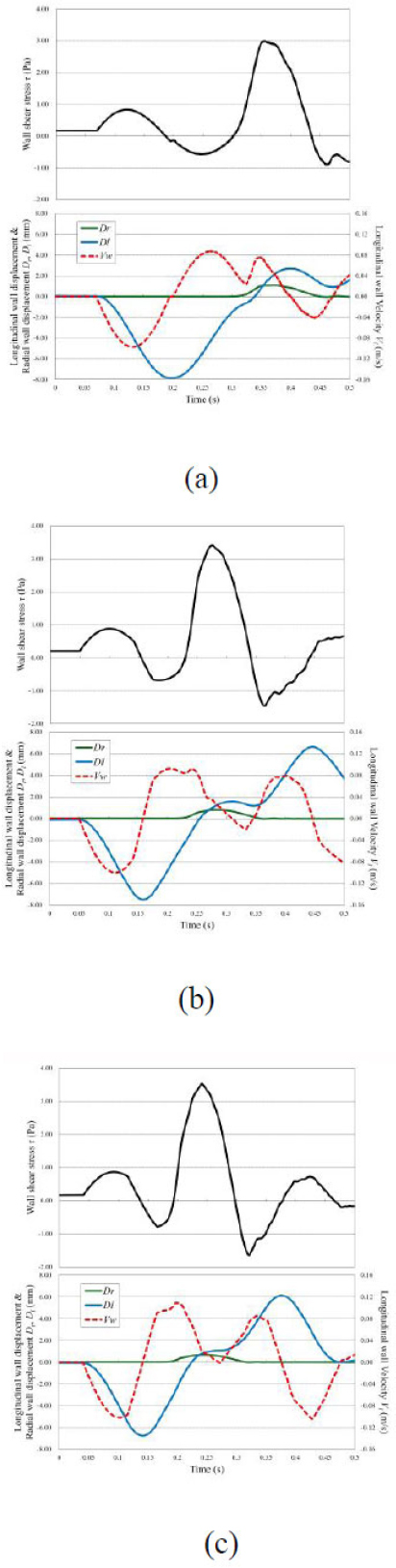
WSS distribution and wave propagation are shown in the arterial model. The WSS τ, radial wall displacement Dr, longitudinal wall displacement Dl, and longitudinal wall velocity Vl observed at z = 1550 mm. (a) E = 0.5 MPa; (b) E = 1.0 MPa; and (c) E = 1.5 MPa.
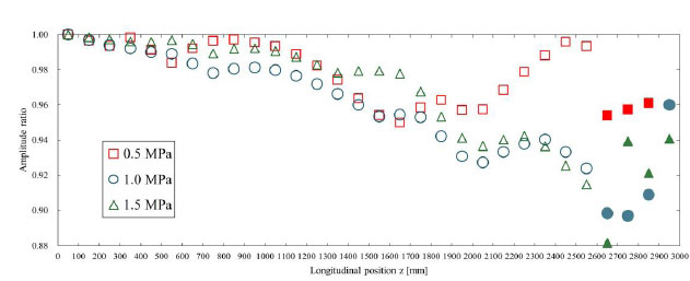
The amplitude ratio is shown for each Young’s modulus. This was calculated with respect to the amplitude of the displacement pulse wave observed at 50 mm. The waveforms where the markers were filled in were processed for separation using the method described in Section 2.4. The displacement waveforms were converted into pressure waveforms as described in Section 2.5 for separation and then reconverted into displacement waveforms.
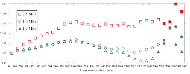
The wavelength ratio is shown for each Young’s modulus. This was calculated with respect to the wavelength of the displacement pulse wave observed at 50 mm. The waveforms where the markers were filled in were processed for separation using the method described in Section 2.4. The displacement waveforms were converted to pressure waveforms as described in Section 2.5 for separation and then reconverted to displacement waveforms.
4.2. Influence of the Frequency of Pulse Waves on the WSS and Waveforms
The period of the inflow velocity was varied to investigate its influence on WSS distribution and the amplitude or wavelength ratio. The Young’s modulus of the arterial wall was fixed at E = 0.5 MPa.
Fig. (9) state that, for all inlet velocity wavelengths, a longitudinal wave Dl propagating at a faster speed than the transverse wave Dr generated wall shear stress. At λ = 125ms, the peak wall shear stress generated by the longitudinal wave was 0.83 Pa, while at λ = 500ms, it was 0.56 Pa. With an increase in the wavelength, the flow rate also increases, leading to greater deformation and a larger amplitude of the longitudinal wave. However, because the flow velocity rises only gradually, the longitudinal wall velocity Vl remains relatively low, resulting in lower wall shear stress from the longitudinal wave. Subsequently, the velocity gradient increased with the propagation of the compression wave, and peak wall shear stress values were observed for each inlet velocity wavelength. It is considered that as the inlet velocity wavelength increases, the flow velocity rises more gradually so that the relative velocity between the wall and the fluid is lower and the peak wall shear stress values become smaller.
As shown in Table 3, regions with a low TAWSS and high OSI were observed under high-frequency inflow conditions. Conversely, regions with a high TAWSS and low OSI were observed under low-frequency inflow conditions. These findings indicate that variations in the pulse wave frequency affect the WSS distribution.
Fig. (10) shows the amplitude ratio of the displacement pulse waves, and Fig. (11) shows the wavelength ratio of the displacement pulse waves. The waveforms at the points indicated by the filled markers were processed for separation using the same method as in the previous section. The attenuation of the amplitude and the diffusion of the wavelength may be attributed to the effects of viscous friction. According to Table 3, under high inlet velocity wavelength conditions, the TAWSS values were high, so it was anticipated that the effects of viscous friction would be significant. However, no clear trend was observed in the amplitude and wavelength of the pulse waveform. This is due to issues with the waveform evaluation method, as described in Section 4.1.
| λ | E | 1,050 mm | 1,550 mm | 2,050 mm |
|---|---|---|---|---|
| TAWSS | 125 ms | 0.4758 | 0.7334 | 0.6394 |
| 250 ms | 0.7079 | 0.8416 | 0.7058 | |
| 500 ms | 0.7070 | 0.7135 | 0.7500 | |
| OSI | 125 ms | 0.1952 | 0.2871 | 0.2095 |
| 250 ms | 0.1951 | 0.2213 | 0.0858 | |
| 500 ms | 0.0965 | 0.0639 | 0.0379 |
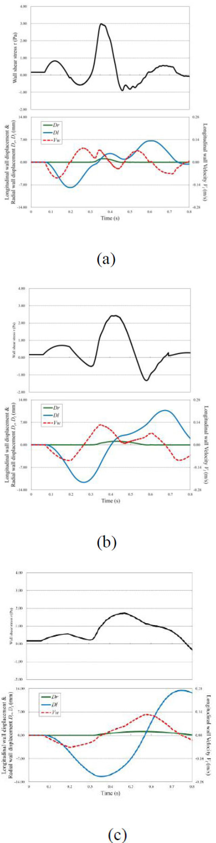
WSS distribution and wave propagation are shown in the arterial model. The WSS T, radial wall displacement Dr, longitudinal wall displacement Dl, and longitudinal wall velocity Vl observed at z = 1,550 mm. (a) λ = 12 5mn; (b) λ = 250ms; and (c) λ = 500 ms.
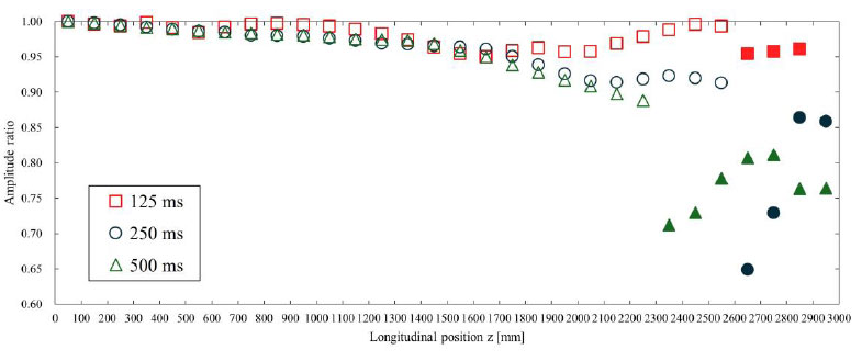
The amplitude ratio is shown for each inlet velocity wavelength. This was calculated with respect to the amplitude of the displacement pulse wave observed at 50 mm. The waveforms where the markers were filled in were processed for separation using the method described in Section 2.4. The displacement waveforms were converted to pressure waveforms as described in Section 2.5 for separation and then reconverted to displacement waveforms.
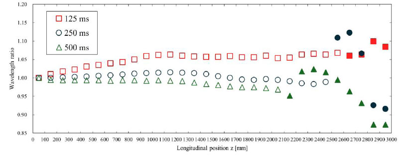
The wavelength ratio is shown for each inlet velocity wavelength. This was calculated with respect to the wavelength of the displacement pulse wave observed at 50 mm. The waveforms where the markers were filled in were processed for separation using the method described in Section 2.4. The displacement waveforms were converted to pressure waveforms as described in Section 2.5 for separation and then reconverted to displacement waveforms.
CONCLUSION
This study investigated the effects of the mechanical properties of arterial walls and the frequency of pulse waves on the WSS and waveforms. In the investigation of the WSS distribution, under conditions of low Young’s modulus or high frequency, the TAWSS values were low and OSI values were high. Conversely, under conditions of high Young’s modulus or low frequency, the TAWSS values were high and OSI values were low. These findings suggest that changes in the mechanical properties of arterial walls associated with the progression of atherosclerosis, as well as differences in the frequency of pulse waves, affect the distribution of WSS.
In the pulse waveform analysis, it was confirmed that the pulse waveform attenuated and diffused during propagation because of viscous friction incorporated in the three-dimensional fluid-structure interaction analysis. Regarding the waveform separation, the accuracy was insufficient, thus highlighting the need for the development of new separation methods that consider the unique effects of three-dimensional analysis. In future studies, refinement of the computational model and pulse wave evaluation methods, including the incorporation of multidimensional parameters such as waveform area, is expected to contribute to the development of reliable diagnostic indicators for atherosclerosis.
AUTHORS' CONTRIBUTIONS
The authors confirm their contribution to the paper as follows: T.F.; Study conception and design; Y.K.: Investigation; All authors reviewed the results and approved the final version of the manuscript.
LIST OF ABBREVIATIONS
| TAWSS | = Time-averaged wall shear stress |
| OSI | = Oscillatory shear index |
| WSS | = Wall shear stress |
AVAILABILITY OF DATA AND MATERIALS
The authors confirm that the data supporting the findings of this research are available within the article.
ACKNOWLEDGEMENTS
The authors would like to thank Altair Engineering for using the RADIOSS as an Altair research support program (ARSP).